14. Test the analysis against known truth
14. Test the analysis against known truth
Simulation can check whether the code an agent has written runs successfully and whether a candidate estimator has desirable statistical properties under conditions relevant to the study. Those are different questions. Code can follow the specification and run without error while producing biased estimates or unreliable uncertainty intervals.
In the heat-and-birthweight example (Chapter 10: The example research project), the agent generates synthetic datasets with known relationships between maternal age, heat exposure, and birthweight. By varying those relationships and repeating the prescribed analysis, it can assess when the method produces reliable estimates and uncertainty intervals.
Check that the code runs from inputs to outputs
Build on the smoke test in Chapter 13: Build a modular analysis workflow. Ask the agent to generate a small synthetic dataset with the variables and formats the code expects, then run it through the complete workflow. For the birthweight example, that means preparing the analysis data, fitting the statistical model, calculating contrasts, and producing the required tables and figures. Have the agent fix errors, missing outputs, and failures between steps before repeating the run.
Synthetic data also let the agent exercise conditions the code needs to handle. For example, it can insert missing birthweights to check that the code applies the prescribed exclusion rule. These functional checks establish whether the code completes the required steps for the supplied inputs. Assessing the estimator’s statistical properties requires repeated datasets with known truth.
Choose the scenarios for evaluating the estimator
The methodological question is how well the proposed analysis performs under conditions that could matter for the study. You identify those conditions; the agent can help turn them into simulation scenarios and explain what each would reveal. In other projects, the simulation scenarios might vary in sample size, the amount of missing data, measurement error, or dependence among observations.
The birthweight example examines three scenarios. In each repetition, the agent generates new birthweights while keeping the 1,200 individuals’ maternal ages, smoking indicators, and heat exposures fixed. All three scenarios retain a curved relationship between maternal age and birthweight. They differ in how heat exposure affects birthweight, while the prescribed analysis allows the heat effect to change linearly with age.
| Scenario | How the data are generated | What the comparison examines |
|---|---|---|
| No heat effect | Heat exposure does not affect birthweight. | Estimates near zero and the frequency of false positives. |
| Linear change with age | The heat effect changes linearly with maternal age, as the analysis assumes. | Performance when the fitted statistical model represents the simulated relationships. |
| Nonlinear change with age | The heat effect also changes quadratically with maternal age. | Performance when the fitted interaction cannot fully represent the simulated relationship. |
Before evaluating the estimator, have the agent check that the data generator can produce plausible values for the study variables. For birthweight, this includes positive values and a defensible distribution and spread. Check relevant constraints between variables too. The example uses positive, right-skewed birthweights; a real study needs scenarios justified by its scientific knowledge and data.
Have the agent calculate the true quantities being estimated directly from the data-generating rules and check those calculations separately from the fitting code. For this example, it calculates mean birthweight at 10 and 5 hot days before adding random variation, then averages the differences over the specified individuals. If the agent uses the same faulty calculation for both the estimate and the value used to check it, the two can agree even though both are wrong.
Have the agent record the approved scenarios, true quantities, number of repetitions, and evaluation criteria in a simulation specification linked from SPECIFICATION.md.1 It should keep simulated inputs and results separate from the primary analysis files.
How the example generates outcomes and calculates truth
The simulation’s performance results concern the fixed covariate values of the 1,200 synthetic individuals. The generator uses positive, right-skewed noise with spread increasing with the conditional mean. The download labels the three scenarios null, main, and curved.
For each scenario, the true sample contrast averages the difference between conditional mean birthweight at 10 and 5 hot days over the saved individuals. Age-specific truth uses the stated age and the sample’s smoking distribution. The estimator includes quadratic age, a linear heat-by-age interaction, and smoking, with HC3 covariance and normal-reference intervals. It is unchanged across scenarios.
A separate calculation can check the implementation of a reported contrast. With age centered at 28, the fitted model’s 10-minus-5-day difference at age 28 is five times its heat coefficient. Ask the agent to compare that expression with the contrast obtained from predictions. This checks the contrast calculation; the repeated simulation assesses its statistical performance.
The project download contains generator code, parameters, independent truth calculations, random seeds, and the simulation specification. A different design may require numerical integration or a large reference population to approximate truth; have the agent record that approximation and its uncertainty.
Have the agent evaluate repeated datasets
Within each scenario, have the agent repeatedly generate a dataset, run the prescribed analysis, and save the estimates, uncertainty intervals, and any failures. The estimator stays unchanged throughout that evaluation. A single estimate can differ from the truth through sampling variation; repeated datasets show how the method behaves across those variations.
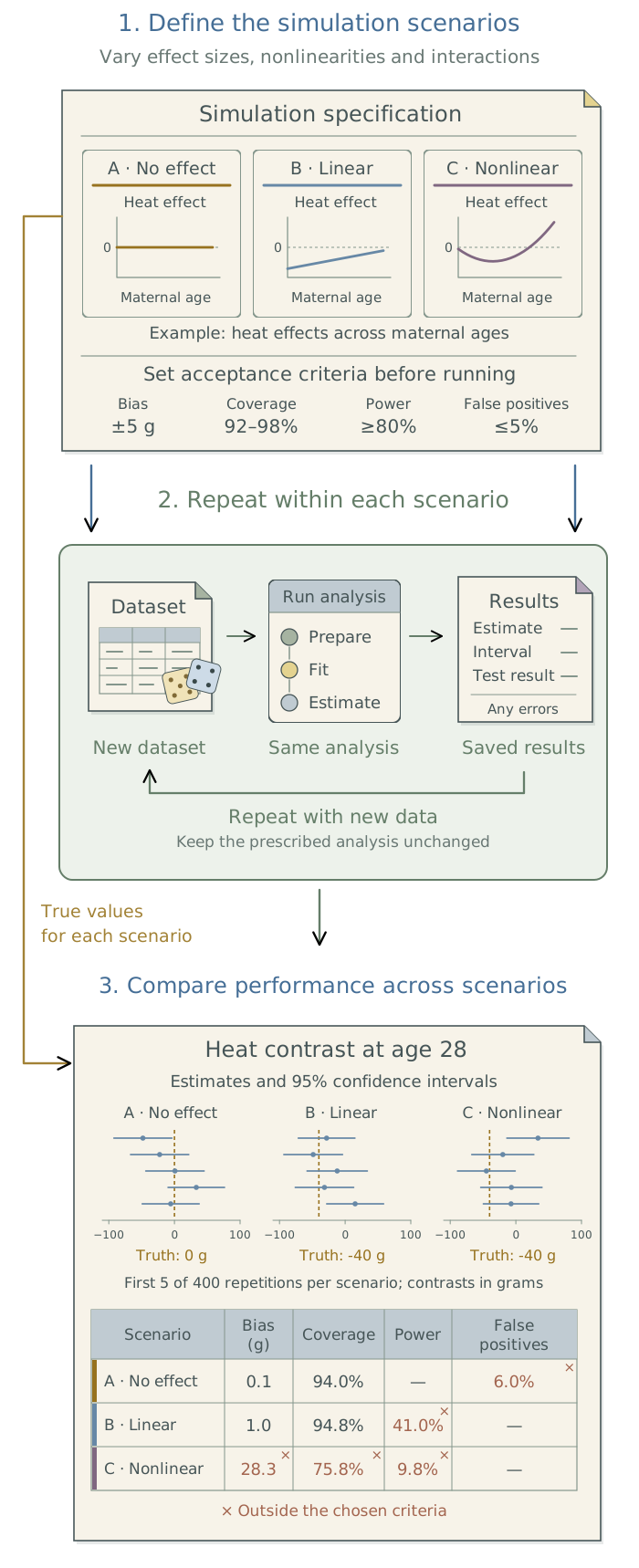
Agree on the performance measures before launching the repetitions. Ask the agent to propose measures suited to the quantities being estimated and any decision rules the study will use. The table below summarizes common choices.
| Measure | What it tells you |
|---|---|
| Bias | Whether estimates are systematically too high or too low. |
| Overall estimation error | How far estimates fall from the truth, accounting for both bias and variation. |
| Interval coverage | How often the uncertainty intervals contain the true value. |
| Interval width | How precise the reported estimates are; high coverage can come from very wide intervals. |
| Power and false-positive rate | How often a specified decision rule detects an effect when one exists, or declares one when none exists. |
| Failure rate | How often the analysis fails to produce an estimate or interval. |
The number of repetitions determines how precisely the simulation estimates statistical performance. With 400 repetitions, an estimated coverage rate near 95 percent has a standard error of about 1.1 percentage points. This is Monte Carlo uncertainty: uncertainty in the estimated performance, rather than in an individual birthweight contrast. More repetitions reduce it. Have the agent choose enough repetitions to distinguish differences that matter for the methodological decision and report the remaining uncertainty.
Using
SPECIFICATION.md, propose simulation scenarios relevant to this study and performance measures for the prescribed estimator. Explain how each dataset will be generated and how the true quantities will be calculated independently of the fitting code. Check that the generator produces plausible values and variability. After I approve the simulation specification, test one complete run, then evaluate repeated datasets in each scenario without changing the estimator. Save estimates, intervals, and failed runs; report performance and its Monte Carlo uncertainty. Keep simulation files separate from the primary analysis and propose any methodological changes for my decision.
Have the agent retain failed runs and report their number alongside the successful ones. If performance summaries exclude failures, it should state that explicitly: results from successful fits alone can make an unstable estimator look reliable.
Use the results to assess and revise the method
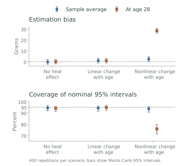
All 1,200 fits in the saved simulation completed without failure: 400 repetitions in each of the three scenarios. Yet when the heat effect changed nonlinearly with age, the estimated difference in mean birthweight between 10 and 5 hot days at maternal age 28 had bias of 28.3 g, and its nominal 95% intervals contained the true value in only 75.8% of repetitions. The code ran successfully, but the prescribed method’s statistical performance was poor for this quantity in this scenario. The sample-average contrast performed much better, so examining only that average would have concealed the problem at age 28.
Read the numerical results
The table shows two of the four reported quantities. Coverage is the proportion of 95% confidence intervals containing the true contrast; the last column reports Monte Carlo uncertainty in that proportion. The project download includes every quantity, repetition, and failure check.
| Scenario | Quantity | Truth (g) | Bias (g) | Coverage | Monte Carlo 95% interval |
|---|---|---|---|---|---|
| No heat effect | Sample average | 0.0 | -0.2 | 94.5% | 91.8%–96.3% |
| No heat effect | Age 28 | 0.0 | 0.1 | 94.0% | 91.2%–95.9% |
| Linear change with age | Sample average | -37.8 | 1.0 | 94.2% | 91.5%–96.1% |
| Linear change with age | Age 28 | -40.0 | 1.0 | 94.8% | 92.1%–96.5% |
| Nonlinear change with age | Sample average | -10.8 | 2.4 | 93.5% | 90.6%–95.5% |
| Nonlinear change with age | Age 28 | -40.0 | 28.3 | 75.8% | 71.3%–79.7% |
When performance is poor, ask the agent to investigate the data generator, truth calculation, and implementation before attributing the problem to the estimator. Preserve the failing runs. A generator that produces impossible values needs correction; an implementation error needs repair; a correctly implemented method that performs poorly may need a scientific revision.
The nonlinear scenario gives a reason to evaluate a more flexible age interaction. If you approve that evaluation, have the agent compare the candidate methods across the relevant scenarios, preserving the original results. An approved change to the prescribed analysis belongs in SPECIFICATION.md, with its reason in METHODOLOGY.md; the agent then reruns the affected analysis and checks.
Simulation supports conclusions about performance under the conditions examined. Chapter 15: Check the agent with independent implementations provides a complementary check: whether separately written implementations carry out the same scientific specification consistently.
Footnotes
Morris, White, and Crowther (2019), “Using simulation studies to evaluate statistical methods”, Statistics in Medicine, provide guidance on specifying a simulation study’s aims, data-generating mechanisms, estimands, methods, and performance measures, and on reporting Monte Carlo uncertainty.↩︎