Stata Introduction

Topics

Stata interface and Do-files
Reading and writing data
Basic summary statistics
Basic graphs
Basic data management
Bivariate analyses

Setup

Software and Materials

Follow the Stata Installation instructions and ensure that you can successfully start Stata.

A handy set of Stata cheat-sheets is available to help you look up and remember command syntax.

Class Structure and organization

Informal — Ask questions at any time. Really!
Collaboration is encouraged - please spend a minute introducing yourself to your neighbors!
If you are using a laptop, you will need to adjust file paths accordingly
Make comments in your Do-file - save on flash drive or email to yourself

Prerequisites

This is an introductory Stata course:

Assumes no prior knowledge of how to use Stata
We do assume you know why you want to learn Stata. If you don’t, and want a comparison of Stata to other statistical software, see our Data Science Tools workshop
Relatively slow-paced

Goals

We will learn about the Stata language by analyzing data from the general social survey (gss). In particular, our goals are to:

Familiarize yourself with the Stata interface
Get data in and out of Stata
Compute statistics and construct graphical displays
Compute new variables and transformations
Perform univariate and bivariate data analyses

Stata basics

GOAL: To learn the basics about Stata, how to interact with Stata, and how to read in and save data. In particular:

What is Stata, why use Stata, and advantages of using Stata
Three ways of interacing with Stata
Set the working directory
Read, save, and write data

What is Stata?

Stata is a statistical software package that you can use to perform data analysis and management, as well as create graphics
Stata is commonly used among health, sociology, and economics researchers, particularly those working with large data sets

Why use Stata?

It is easy to learn and is supported by a wide range of introductory textbooks
It offers a wide range of statistical models in a consistent interface
It presents results in a clear format
It has very good built-in help documentation and a broad user community where you can seek help
Student and other discount packages are available at reasonable cost

How does Stata work?

When Stata is running, variables, data, etc., are stored in memory. The user can use clear command to clear up memory before running further commands, unless they want to save their changes in the original dataset or a new dataset.

Interfaces

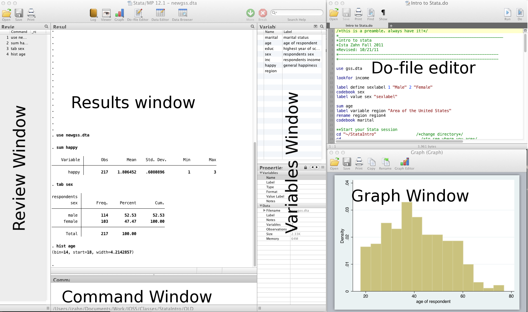
Review and Variable windows can be closed (user preference)
Command window can be shortened (recommended)

GUI and command window

There are two ways of interacting with Stata that will not result in a saveable record of what you have done:

GUI. The Graphical User Interface (GUI) allows you to perform analyses using drop-down menus, rather than writing code. This can be easier for first time users and Stata will helpfully display the command and proper syntax for the operation that you have selected. However, we strongly recommend not using the GUI, since it does not produce a script — a record of what you have done — and thus leads to analyses that are unreproducible.
Command window. From the command window you can type commands to manage and analyze your data.
- The advantage is that you can quickly produce output of a single command.
- The disadvantage is that you cannot store your syntax in a script to reproduce in the future.

Do-file

The third way of interacting with Stata does provide you with a saveable record of your work:

Do-file. A do-file is a plain text file within which you can write and save commands for later use. There are several advantages to using a do-file and we strongly recommend that you always interact with Stata in this way:
- Allows you to submit more than one command to Stata at once.
- Has specialized features for programmers such as syntax highlighting, code folding, autocompletion, and bookmarks to important lines in your code, brace matching, and more.
- With a do-file, it is easy to save, review, change, and share your code with others — including your future self!

Here are some resources for learning more about Stata and do-files:

Stata help

To get help in Stata type help followed by topic or command, e.g., help codebook.

Syntax rules

Most Stata commands follow the same basic syntax: Command varlist, options.
Use comments liberally — start with a comment describing your do-file and use comments throughout
- Use * to comment a line and // for in-line comments
- Use /// to break varlists over multiple lines

Exercise 0

Launch the Stata program (MP or SE, does not matter unless doing computationally intensive work) * Open up a new do-file * Run our first Stata code!

Try to get Stata to say “Hello World!”. Search help display.

##

Try to get Stata to break “Hello World!” over two lines:

##

Click for Exercise 0 Solution

Try to get Stata to say “Hello World!”. Search help display.

disp "Hello " "World!" // 'disp' is short for 'display'

Try to get Stata to break “Hello World!” over two lines:

disp "Hello" ///
     " World!"

Working directory

print current working directory

pwd

change working directory

cd C:\Users\yiw640\Desktop\StataIntro\

A note about file path names

If your file path has no spaces in the name (that means all directories, folders, file names, etc. can have no spaces), you can write the file path as it is
If there are spaces, you need to put your file path name in quotes
Best to get in the habit of quoting file paths

Reading data

Data file commands

Next, we want to open our data file
Open / save data sets with use and save:

// open the gss.dta data set 
use gss.dta, clear

// save data file
save newgss.dta, replace // `replace` option means OK to overwrite existing file

Where’s my data?

Data editor (browse)
Data editor (edit)
- Using the data editor is discouraged (why?)
Always keep any changes to your data in your do-file
Avoid temptation of making manual changes by viewing data via the browser rather than editor

Reading non-Stata data

Import / export delimited text files

// import data from a .csv file
import delimited gss.csv, clear

// save data to a .csv file
export delimited gss_new.csv, replace

Import / export Excel files

// import/export Excel files
clear
import excel gss.xlsx
export excel gss_new, replace

What if my data is from another statistical software program?

SPSS/PASW will allow you to save your data as a Stata file
- Go to: file -> save as -> Stata (use most recent version available)
- Then you can just go into Stata and open it
Another option is StatTransfer, a program that converts data from/to many common formats, including SAS, SPSS, Stata, and many more.

Statistics & graphs

GOAL: To learn the basic commands to review, inspect, and plot data in Stata. In particular:

Learn more about the variables in our dataset — using the describe, codebook, and browse commands
Produce univariate distributions using histogram, and bivariate distribution using scatterplot
Tabulate or summarize your data within certain groups using bysort

The most frequently used commands for reviewing and inspecting data are summarized below:

Command	Description
`describe`	labels, storage type etc.
`sum`	statistical summary (mean, sd, min/max etc.)
`codebook`	storage type, unique values, labels
`list`	print actual values
`tab`	(cross) tabulate variables
`browse`	view the data in a spreadsheet-like window

First, let’s ask Stata for help about these commands:

help sum

use gss.dta, clear

sum educ // statistical summary of education

codebook region // information about how region is coded

tab sex // numbers of male and female participants

Note — if you run these commands without specifying variables, Stata will produce output for every variable.

Basic graphing commands

Univariate distribution(s) using hist:

// Histograms 
hist educ

// histogram with normal curve; see `help hist` for other options
hist age, normal

View bivariate distributions with scatterplots:

// scatterplots 
twoway (scatter educ age)

graph matrix educ age inc

The `by` command

Sometimes, you’d like to generate output based on different categories of a grouping variable, for example:

you want to know the distribution of happiness seperately for men and women: tabulate happy by sex:

bysort sex: tab happy

you want to know the mean level of education for different marital status: summarize education by marital status (marital):

bysort marital: sum educ

Save your changes to the original gss.dta dataset.

Exercise 1

We are using The Generations of Talent Study (talent.dta) to practice reading in data, plotting data, and calculating descriptive statistics. The dataset includes information on quality of employment as experienced by today’s multigenerational workforces. Here is a codebook of a subset of variables:

Variable name	Label
job	type of main job
workload	how long hours do you work per week
otherjob	do you have other paid jobs beside main job
schedule	which best describes your work schedule
fulltime	Does your employer consider you a full-time or part-time employee
B3A	How important are the following to you? Your work
B3B	How important are the following to you? Your family
B3C	How important are the following to you? Your friends
marital	Which of the following best describes your current marital status
I3	Sex/gender
income	What was your total household income during last year

Create a new do-file for the following exercise prompts. After the exercise save the do-file to your working directory.

Read in the dataset talent.dta:

##

Examine a few selected variables using the describe, sum and codebook commands:

##

Produce a histogram of hours worked (workload) and add a normal curve:

##

Summarize the total household income last year (income) by marital status (marital):

##

Cross-tabulate marital status (marital) with respondents’ type of main job (job):

##

Click for Exercise 1 Solution

Read in the dataset talent.dta:

use talent.dta, clear

Examine a few selected variables using the describe, sum and codebook commands:

describe workperweek
tab I3
sum income
codebook job

Produce a histogram of hours worked (workload) and add a normal curve:

hist workload, normal

Summarize the total household income last year (income) by marital status (marital):

bysort marital: sum income

Cross-tabulate marital status (marital) with respondents’ type of main job (job):

bysort job: tab marital

Basic data management

GOAL: To learn how to add variable labels and value labels, as well as create new variables in Stata. In particular:

Use label and rename to set / modify variable and value labels
Use generate and replace to create a new variables based on values of existing variables/recode a variable

Variable & value labels

Variable labels

It’s good practice to ALWAYS label every variable, no matter how insignificant it may seem.

// Labelling and renaming 
// Label variable inc "household income"
label var inc "household income"

// change the name "educ" to "education"
rename educ education

// you can search names and labels with `lookfor`
lookfor household

Value labels

Value labels are a little more complicated, with a two step process: define a value label, then assign defined label to variable(s)

// define a value label for sex 
label define mySexLabel 1 "Male" 2 "Female"

// assign our label set to the sex variable
label values sex mySexLabel

Working on subsets

It is often useful to select just those rows of your data where some condition holds — for example select only rows where sex is 1 (male). The following operators allow you to do this:

Operator	Meaning
==	equal to
!=	not equal to
>	greater than
>=	greater than or equal to
<	less than
<=	less than or equal to
&	and
\|	or

Note the double equals signs for testing equality.

Generating & replacing variables

Often, it can be useful to start with a new variable composed of blank values and fill values in based on the values of existing variables:

// generate a column of missings
gen age_wealth = .

// Next, start adding your qualifications
replace age_wealth=1 if age < 30 & inc < 10
replace age_wealth=2 if age < 30 & inc > 10
replace age_wealth=3 if age > 30 & inc < 10
replace age_wealth=4 if age > 30 & inc > 10

Exercise 2

Open the talent.dta data, use the basic data management tools we have learned to add labels and generate new variables:

Tabulate the variable, marital status (marital), with and without labels:

##

Summarize the total household income last year (income) for married individuals only:

##

Generate a new overwork dummy variable from the original variable workperweek that will take on a value of 1 if a person works more than 40 hours per week, and 0 if a person works equal to or less than 40 hours per week:

##

Generate a new marital_dummy dummy variable from the original variable marital that will take on a value of 1 if a person is either married or partnered and 0 otherwise:

##

Rename the Sex variable and give it a more intuitive name:

##

Give a variable label and value labels for the variable overwork:

##

Generate a new variable called work_family and code it as 2 if a respondent perceived work to be more important than family, 1 if a respondent perceived family to be more important than work, and 0 if the two are of equal importance:

##

Save the changes to newtalent.dta:

##

Click for Exercise 2 Solution

Open the talent.dta data, use the basic data management tools we have learned to add labels and generate new variables:

Tabulate the variable, marital status (marital), with and without labels:

use talent.dta, clear

tab marital
tab marital, nol

Summarize the total household income last year (income) for married individuals only:

summarize income if marital == 1

Generate a new overwork dummy variable from the original variable workperweek that will take on a value of 1 if a person works more than 40 hours per week, and 0 if a person works equal to or less than 40 hours per week:

gen overwork = .
replace overwork = 1 if workperweek > 40
replace overwork = 0 if workperweek <= 40
tab overwork

Generate a new marital_dummy dummy variable from the original variable marital that will take on a value of 1 if a person is either married or partnered and 0 otherwise:

gen marital_dummy = .
replace marital_dummy = 1 if marital == 1 | marital == 2
replace marital_dummy = 0 if marital != 1 & marital != 2
tab marital_dummy

Rename the Sex variable and give it a more intuitive name:

rename I3 Sex

Give a variable label and value labels for the variable overwork:

label variable overwork "whether someone works more than 40 hours per week"
label define overworklabel 1 "Yes" 0 "No"
label values overwork overworklabel

Generate a new variable called work_family and code it as 2 if a respondent perceived work to be more important than family, 1 if a respondent perceived family to be more important than work, and 0 if the two are of equal importance:

gen work_family = .
replace work_family = 2 if B3A > B3B
replace work_family = 1 if B3A < B3B
replace work_family = 0 if B3A == B3B

Save the changes to newtalent.dta:

save newtalent.dta, replace

Bivariate analyses

GOAL: To learn the basic commands for performing the following bivariate analyses.

Chi-squared test
Independent group t-test
One-way ANOVA

Chi-squared test

The Chi-squared statistic is commonly used for testing relationships between categorical variables.

In Stata, both the tabulate and tabi commands conduct the Pearson’s Chi-square test.

The tabulate (may be abbreviated as tab) command produces one- or two-way frequency tables given one or two raw variables
The tabi command is used to re-analyze a published table without access to the raw data
These commands also can run a Chi-square test using the chi2 option:

tab sex happy, chi2

The first command below conducts a Chi-square test for a 2x2 table, while the second and third commands run the test for 3x2 and 2x3 tables, respectively.

tabi 33 48 \ 37 52, chi2
tabi 33 48 \ 37 52 \ 36 42, chi2
tabi 33 48 26 \ 37 52 38, chi2

t-test

The t-test is a type of inferential statistic that can be used to determine if a sample mean differs from a postulated population mean, or if two sample means came from the same population.

Types of t-test:

Independent group t-test: designed to compare means of same variable between two groups. For example, test GRE scores between students from two countries
Other t-tests: single sample t-test; paired t-test. More details see: https://www.stata.com/manuals13/rttest.pdf

In our example, we conduct an independent group t-test to compare mean income (inc) between males and females (sex):

ttest inc, by(sex)

One-way ANOVA

One-way ANOVA allows us to test the equality of more than two sample means (i.e., whether they could plausibly have come from the same population). For example, our dataset contains income (inc) and four regions of the country (region). Using one-way ANOVA, we can simultaneously test the equality of the income means across all regions.

oneway inc region

Now we find evidence that the means are different, but perhaps we are interested only in testing whether the means for the North (region==1) and South (region==4) are different. We also use one-way ANOVA, which in this case would be equivelant to the independent group t-test:

oneway inc region if region==1 | region==4

Exercise 3

Open the newtalent.dta data, use the basic data management tools we have learned to conduct bivariate analysis.

Test the relationship between two variables sex and type of main job (job):

##

Test if there is a significant difference in hours worked per week (workload) and sex:

##

Test if there is a significant difference in hours worked per week (workload) and marital status (marital):

##

Click for Exercise 3 Solution