R Regression Models

Topics

Formula interface for model specification
Function methods for extracting quantities of interest from models
Contrasts to test specific hypotheses
Model comparisons
Predicted marginal effects
Modeling continuous and binary outcomes
Modeling clustered data

Setup

Software and Materials

Follow the R Installation instructions and ensure that you can successfully start RStudio.

Class Structure

Informal - Ask questions at any time. Really!

Collaboration is encouraged - please spend a minute introducing yourself to your neighbors!

Prerequisites

This is an intermediate R course:

Assumes working knowledge of R
Relatively fast-paced
This is not a statistics course! We will teach you how to fit models in R, but we assume you know the theory behind the models.

Goals

We will learn about the R modeling ecosystem by fitting a variety of statistical models to different datasets. In particular, our goals are to learn about:

Modeling workflow
Visualizing and summarizing data before modeling
Modeling continuous outcomes
Modeling binary outcomes
Modeling clustered data

We will not spend much time interpreting the models we fit, since this is not a statistics workshop. But, we will walk you through how model results are organized and orientate you to where you can find typical quantities of interest.

Launch an R session

Start RStudio and create a new project:

On Mac, RStudio will be in your applications folder. On Windows, click the start button and search for RStudio.
In RStudio go to File -> New Project. Choose Existing Directory and browse to the workshop materials directory on your desktop. This will create an .Rproj file for your project and will automaticly change your working directory to the workshop materials directory.
Choose File -> Open File and select the file with the word “BLANK” in the name.

Packages

You should have already installed the tidyverse and rmarkdown packages onto your computer before the workshop — see R Installation. Now let’s load these packages into the search path of our R session.

library(tidyverse)
library(rmarkdown)

Finally, lets install some packages that will help with modeling:

# install.packages("lme4")
library(lme4)  # for mixed models

# install.packages("emmeans")
library(emmeans)  # for marginal effects

# install.packages("effects")
library(effects)  # for predicted marginal means

Modeling workflow

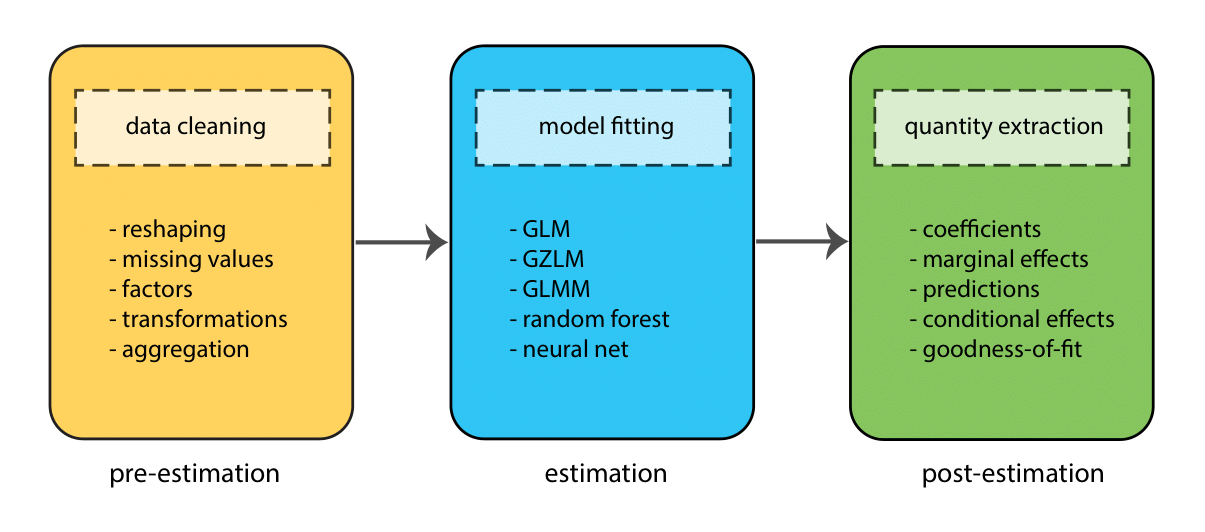
Before we delve into the details of how to fit models in R, it’s worth taking a step back and thinking more broadly about the components of the modeling process. These can roughly be divided into 3 stages:

Pre-estimation
Estimation
Post-estimaton

At each stage, the goal is to complete a different task (e.g., to clean data, fit a model, test a hypothesis), but the process is sequential — we move through the stages in order (though often many times in one project!)

Throughout this workshop we will go through these stages several times as we fit different types of model.

R modeling ecosystem

There are literally hundreds of R packages that provide model fitting functionality. We’re going to focus on just two during this workshop — stats, from Base R, and lme4. It’s a good idea to look at CRAN Task Views when trying to find a modeling package for your needs, as they provide an extensive curated list. But, here’s a more digestable table showing some of the most popular packages for particular types of model.

Models	Packages
Generalized linear	`stats`, `biglm`, `MASS`, `robustbase`
Mixed effects	`lme4`, `nlme`, `glmmTMB`, `MASS`
Econometric	`pglm`, `VGAM`, `pscl`, `survival`
Bayesian	`brms`, `blme`, `MCMCglmm`, `rstan`
Machine learning	`mlr`, `caret`, `h2o`, `tensorflow`

Before fitting a model

GOAL: To learn about the data by creating summaries and visualizations.

One important part of the pre-estimation stage of model fitting, is gaining an understanding of the data we wish to model by creating plots and summaries. Let’s do this now.

Load the data

List the data files we’re going to work with:

list.files("dataSets")

## [1] "Exam.rds"          "NatHealth2008MI"   "NatHealth2011.rds"
## [4] "states.rds"

We’re going to use the states data first, which originally appeared in Statistics with Stata by Lawrence C. Hamilton.

  # read the states data
  states <- read_rds("dataSets/states.rds")

  # look at the last few rows
  tail(states)

##            state  region     pop  area density metro waste energy miles toxic
## 46       Vermont N. East  563000  9249   60.87  23.4  0.69    232  10.4  1.81
## 47      Virginia   South 6187000 39598  156.25  72.5  1.45    306   9.7 12.87
## 48    Washington    West 4867000 66582   73.10  81.7  1.05    389   9.2  8.51
## 49 West Virginia   South 1793000 24087   74.44  36.4  0.95    415   8.6 21.30
##    green house senate csat vsat msat percent expense income high college
## 46 15.17    85     94  890  424  466      68    6738 34.717 80.8    24.3
## 47 18.72    33     54  890  424  466      60    4836 38.838 75.2    24.5
## 48 16.51    52     64  913  433  480      49    5000 36.338 83.8    22.9
## 49 51.14    48     57  926  441  485      17    4911 24.233 66.0    12.3
##  [ reached 'max' / getOption("max.print") -- omitted 2 rows ]

Here’s a table that describes what each variable in the dataset represents:

Variable	Description
csat	Mean composite SAT score
expense	Per pupil expenditures
percent	% HS graduates taking SAT
income	Median household income, $1,000
region	Geographic region: West, N. East, South, Midwest
house	House ’91 environ. voting, %
senate	Senate ’91 environ. voting, %
energy	Per capita energy consumed, Btu
metro	Metropolitan area population, %
waste	Per capita solid waste, tons

Examine the data

Start by examining the data to check for problems.

  # summary of expense and csat columns, all rows
  states_ex_sat <- states %>% 
      select(expense, csat)
  
  summary(states_ex_sat)

##     expense          csat       
##  Min.   :2960   Min.   : 832.0  
##  1st Qu.:4352   1st Qu.: 888.0  
##  Median :5000   Median : 926.0  
##  Mean   :5236   Mean   : 944.1  
##  3rd Qu.:5794   3rd Qu.: 997.0  
##  Max.   :9259   Max.   :1093.0

  # correlation between expense and csat
  cor(states_ex_sat, use = "pairwise")

##            expense       csat
## expense  1.0000000 -0.4662978
## csat    -0.4662978  1.0000000

Plot the data

Plot the data to look for multivariate outliers, non-linear relationships etc.

  # scatter plot of expense vs csat
  qplot(x = expense, y = csat, geom = "point", data = states_ex_sat)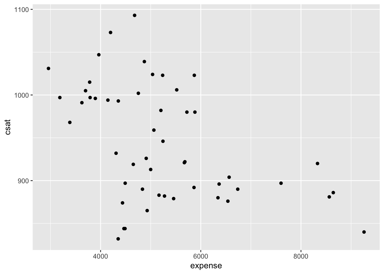

Obviously, in a real project, you would want to spend more time investigating the data, but we’ll now move on to modeling.

Models with continuous outcomes

GOAL: To learn about the R modeling ecosystem by fitting ordinary least squares (OLS) models. In particular:

Formula representation of model specification
Model classes
Function methods
Model comparison

Once the data have been inspected and cleaned, we can start estimating models. The simplest models (but those with the most assumptions) are those for continuous and unbounded outcomes. Typically, for these outcomes, we’d use a model estimated using Ordinary Least Lquares (OLS), which in R can be fit with the lm() (linear model) function.

To fit a model in R, we first have to convert our theoretical model into a formula — a symbolic representation of the model in R syntax:

# formula for model specification
outcome ~ pred1 + pred2 + pred3

# NOTE the ~ is a tilde

For example, the following theoretical model predicts SAT scores based on per-pupil expenditures:

\[ SATscores_i = \beta_{0}1 + \beta_1expenditures_i + \epsilon_i \]

We can use lm() to fit this model:

  # fit our regression model
  sat_mod <- lm(csat ~ 1 + expense, # regression formula
                data = states) # data 

  # look at the basic printed output
  sat_mod

## 
## Call:
## lm(formula = csat ~ 1 + expense, data = states)
## 
## Coefficients:
## (Intercept)      expense  
##  1060.73244     -0.02228

The default printed output from the fitted model is very austere — just point estimates of the coefficients. We can get more information by passing the fitted model object to the summary() function, which provides standard errors, test statistics, and p-values for individual coefficients, as well as goodness-of-fit measures for the overall model.

  # get more informative summary information 
  summary(sat_mod)

## 
## Call:
## lm(formula = csat ~ 1 + expense, data = states)
## 
## Residuals:
##      Min       1Q   Median       3Q      Max 
## -131.811  -38.085    5.607   37.852  136.495 
## 
## Coefficients:
##               Estimate Std. Error t value Pr(>|t|)    
## (Intercept)  1.061e+03  3.270e+01   32.44  < 2e-16 ***
## expense     -2.228e-02  6.037e-03   -3.69 0.000563 ***
## ---
## Signif. codes:  0 '***' 0.001 '**' 0.01 '*' 0.05 '.' 0.1 ' ' 1
## 
## Residual standard error: 59.81 on 49 degrees of freedom
## Multiple R-squared:  0.2174, Adjusted R-squared:  0.2015 
## F-statistic: 13.61 on 1 and 49 DF,  p-value: 0.0005631

If we just want to inspect the coefficients, we can further pipe the summary output into the function coef() to obtain just the table of coefficients.

  # show only the regression coefficients table 
  summary(sat_mod) %>% coef()

##                  Estimate   Std. Error   t value     Pr(>|t|)
## (Intercept) 1060.73244395 32.700896736 32.437412 8.878411e-35
## expense       -0.02227565  0.006037115 -3.689783 5.630902e-04

Why is the association between expense & SAT scores negative?

Many people find it surprising that the per-capita expenditure on students is negatively related to SAT scores. The beauty of multiple regression is that we can try to pull these apart. What would the association between expense and SAT scores be if there were no difference among the states in the percentage of students taking the SAT?

  lm(csat ~ 1 + expense + percent, data = states) %>% 
  summary()

## 
## Call:
## lm(formula = csat ~ 1 + expense + percent, data = states)
## 
## Residuals:
##     Min      1Q  Median      3Q     Max 
## -62.921 -24.318   1.741  15.502  75.623 
## 
## Coefficients:
##               Estimate Std. Error t value Pr(>|t|)    
## (Intercept) 989.807403  18.395770  53.806  < 2e-16 ***
## expense       0.008604   0.004204   2.046   0.0462 *  
## percent      -2.537700   0.224912 -11.283 4.21e-15 ***
## ---
## Signif. codes:  0 '***' 0.001 '**' 0.01 '*' 0.05 '.' 0.1 ' ' 1
## 
## Residual standard error: 31.62 on 48 degrees of freedom
## Multiple R-squared:  0.7857, Adjusted R-squared:  0.7768 
## F-statistic: 88.01 on 2 and 48 DF,  p-value: < 2.2e-16

The `lm` class & methods

Okay, we fitted our model. Now what? Typically, the main goal in the post-estimation stage of analysis is to extract quantities of interest from our fitted model. These quantities could be things like:

Testing whether one group is different on average from another group
Generating average response values from the model for interesting combinations of predictor values
Calculating interval estimates for particular coefficients

But before we can do any of that, we need to know more about what a fitted model actually is, what information it contains, and how we can extract from it information that we want to report.

To understand what a fitted model object is and what information we can extract from it, we need to know about the concepts of class and method. A class defines a type of object, describing what properties it possesses, how it behaves, and how it relates to other types of objects. Every object must be an instance of some class. A method is a function associated with a particular type of object.

Let’s start by examining the class of the model object:

  # what class of object is the fitted model?
  class(sat_mod)

## [1] "lm"

We can see that the fitted model object is of class lm, which stands for linear model. What quantities are stored within this model object?

  # what are the elements stored within the fitted model object?
  names(sat_mod)

##  [1] "coefficients"  "residuals"     "effects"       "rank"         
##  [5] "fitted.values" "assign"        "qr"            "df.residual"  
##  [9] "xlevels"       "call"          "terms"         "model"

We can see that 12 different things are stored within a fitted model of class lm. In what structure are these quantities organized?

  # what is the structure of the fitted model object?
  str(sat_mod)

## List of 12
##  $ coefficients : Named num [1:2] 1060.7324 -0.0223
##   ..- attr(*, "names")= chr [1:2] "(Intercept)" "expense"
##  $ residuals    : Named num [1:51] 11.1 44.8 -32.7 26.7 -63.7 ...
##   ..- attr(*, "names")= chr [1:51] "1" "2" "3" "4" ...
##  $ effects      : Named num [1:51] -6742.2 220.7 -31.7 29.7 -63.2 ...
##   ..- attr(*, "names")= chr [1:51] "(Intercept)" "expense" "" "" ...
##  $ rank         : int 2
##  $ fitted.values: Named num [1:51] 980 875 965 978 961 ...
##   ..- attr(*, "names")= chr [1:51] "1" "2" "3" "4" ...
##  $ assign       : int [1:2] 0 1
##  $ qr           :List of 5
##   ..$ qr   : num [1:51, 1:2] -7.14 0.14 0.14 0.14 0.14 ...
##   .. ..- attr(*, "dimnames")=List of 2
##   .. .. ..$ : chr [1:51] "1" "2" "3" "4" ...
##   .. .. ..$ : chr [1:2] "(Intercept)" "expense"
##   .. ..- attr(*, "assign")= int [1:2] 0 1
##   ..$ qraux: num [1:2] 1.14 1.33
##   ..$ pivot: int [1:2] 1 2
##   ..$ tol  : num 1e-07
##   ..$ rank : int 2
##   ..- attr(*, "class")= chr "qr"
##  $ df.residual  : int 49
##  $ xlevels      : Named list()
##  $ call         : language lm(formula = csat ~ 1 + expense, data = states)
##  $ terms        :Classes 'terms', 'formula'  language csat ~ 1 + expense
##   .. ..- attr(*, "variables")= language list(csat, expense)
##   .. ..- attr(*, "factors")= int [1:2, 1] 0 1
##   .. .. ..- attr(*, "dimnames")=List of 2
##   .. .. .. ..$ : chr [1:2] "csat" "expense"
##   .. .. .. ..$ : chr "expense"
##   .. ..- attr(*, "term.labels")= chr "expense"
##   .. ..- attr(*, "order")= int 1
##   .. ..- attr(*, "intercept")= int 1
##   .. ..- attr(*, "response")= int 1
##   .. ..- attr(*, ".Environment")=<environment: R_GlobalEnv> 
##   .. ..- attr(*, "predvars")= language list(csat, expense)
##   .. ..- attr(*, "dataClasses")= Named chr [1:2] "numeric" "numeric"
##   .. .. ..- attr(*, "names")= chr [1:2] "csat" "expense"
##  $ model        :'data.frame':   51 obs. of  2 variables:
##   ..$ csat   : int [1:51] 991 920 932 1005 897 959 897 892 840 882 ...
##   ..$ expense: int [1:51] 3627 8330 4309 3700 4491 5064 7602 5865 9259 5276 ...
##   ..- attr(*, "terms")=Classes 'terms', 'formula'  language csat ~ 1 + expense
##   .. .. ..- attr(*, "variables")= language list(csat, expense)
##   .. .. ..- attr(*, "factors")= int [1:2, 1] 0 1
##   .. .. .. ..- attr(*, "dimnames")=List of 2
##   .. .. .. .. ..$ : chr [1:2] "csat" "expense"
##   .. .. .. .. ..$ : chr "expense"
##   .. .. ..- attr(*, "term.labels")= chr "expense"
##   .. .. ..- attr(*, "order")= int 1
##   .. .. ..- attr(*, "intercept")= int 1
##   .. .. ..- attr(*, "response")= int 1
##   .. .. ..- attr(*, ".Environment")=<environment: R_GlobalEnv> 
##   .. .. ..- attr(*, "predvars")= language list(csat, expense)
##   .. .. ..- attr(*, "dataClasses")= Named chr [1:2] "numeric" "numeric"
##   .. .. .. ..- attr(*, "names")= chr [1:2] "csat" "expense"
##  - attr(*, "class")= chr "lm"

We can see that the fitted model object is a list structure (a container that can hold different types of objects). What have we learned by examining the fitted model object? We can see that the default output we get when printing a fitted model of class lm is only a small subset of the information stored within the model object. How can we access other quantities of interest from the model?

We can use methods (functions designed to work with specific classes of object) to extract various quantities from a fitted model object (sometimes these are referred to as extractor functions). A list of all the available methods for a given class of object can be shown by using the methods() function with the class argument set to the class of the model object:

  # methods for class `lm`
  methods(class = class(sat_mod))

##  [1] add1           alias          anova          case.names     coerce        
##  [6] confint        cooks.distance deviance       dfbeta         dfbetas       
## [11] drop1          dummy.coef     Effect         effects        emm_basis     
## [16] extractAIC     family         formula        fortify        hatvalues     
## [21] influence      initialize     kappa          labels         logLik        
## [26] model.frame    model.matrix   nobs           plot           predict       
## [31] print          proj           qqnorm         qr             recover_data  
## [36] residuals      rstandard      rstudent       show           simulate      
## [41] slotsFromS3    summary        variable.names vcov          
## see '?methods' for accessing help and source code

There are 44 methods available for the lm class. We’ve already seen the summary() method for lm, which is always a good place to start after fitting a model:

  # summary table
  summary(sat_mod)

## 
## Call:
## lm(formula = csat ~ 1 + expense, data = states)
## 
## Residuals:
##      Min       1Q   Median       3Q      Max 
## -131.811  -38.085    5.607   37.852  136.495 
## 
## Coefficients:
##               Estimate Std. Error t value Pr(>|t|)    
## (Intercept)  1.061e+03  3.270e+01   32.44  < 2e-16 ***
## expense     -2.228e-02  6.037e-03   -3.69 0.000563 ***
## ---
## Signif. codes:  0 '***' 0.001 '**' 0.01 '*' 0.05 '.' 0.1 ' ' 1
## 
## Residual standard error: 59.81 on 49 degrees of freedom
## Multiple R-squared:  0.2174, Adjusted R-squared:  0.2015 
## F-statistic: 13.61 on 1 and 49 DF,  p-value: 0.0005631

We can use the confint() method to get interval estimates for our coefficients:

  # confidence intervals
  confint(sat_mod)

##                    2.5 %        97.5 %
## (Intercept) 995.01753164 1126.44735626
## expense      -0.03440768   -0.01014361

And we can use the anova() method to get an ANOVA-style table of the model:

  # ANOVA table
  anova(sat_mod)

## Analysis of Variance Table
## 
## Response: csat
##           Df Sum Sq Mean Sq F value    Pr(>F)    
## expense    1  48708   48708  13.614 0.0005631 ***
## Residuals 49 175306    3578                      
## ---
## Signif. codes:  0 '***' 0.001 '**' 0.01 '*' 0.05 '.' 0.1 ' ' 1

How does R know which method to call for a given object? R uses generic functions, which provide access to the methods. Method dispatch takes place based on the class of the first argument to the generic function. For example, for the generic function summary() and an object of class lm, the method dispatched will be summary.lm(). Here’s a schematic that shows the process of method dispatch in action:

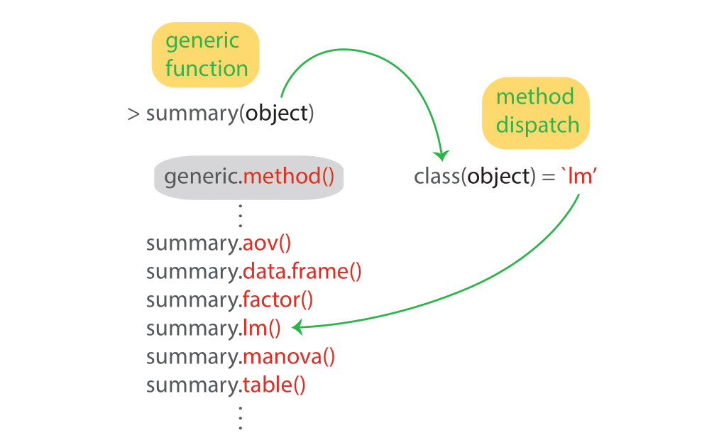
Function methods always take the form generic.method(). Let’s look at all the methods for the generic summary() function:

  # methods for generic `summary()` function
  methods("summary")

##   [1] summary,ANY-method             summary,DBIObject-method      
##   [3] summary,diagonalMatrix-method  summary,sparseMatrix-method   
##   [5] summary.aareg*                 summary.allFit*               
##   [7] summary.aov                    summary.aovlist*              
##   [9] summary.aspell*                summary.cch*                  
##  [11] summary.check_packages_in_dir* summary.connection            
##  [13] summary.corAR1*                summary.corARMA*              
##  [15] summary.corCAR1*               summary.corCompSymm*          
##  [17] summary.corExp*                summary.corGaus*              
##  [19] summary.corIdent*              summary.corLin*               
##  [21] summary.corNatural*            summary.corRatio*             
##  [23] summary.corSpher*              summary.corStruct*            
##  [25] summary.corSymm*               summary.coxph*                
##  [27] summary.coxph.penal*           summary.data.frame            
##  [29] summary.Date                   summary.DBIrepdesign*         
##  [31] summary.DBIsvydesign*          summary.default               
##  [33] summary.Duration*              summary.ecdf*                 
##  [35] summary.eff*                   summary.efflatent*            
##  [37] summary.efflist*               summary.effpoly*              
##  [39] summary.emm_list*              summary.emmGrid*              
##  [41] summary.factor                 summary.ggplot*               
##  [43] summary.glht*                  summary.glht_list*            
##  [45] summary.glm                    summary.gls*                  
##  [47] summary.haven_labelled*        summary.hcl_palettes*         
##  [49] summary.infl*                  summary.Interval*             
##  [51] summary.lm                     summary.lme*                  
##  [53] summary.lmList*                summary.lmList4*              
##  [55] summary.loess*                 summary.loglm*                
##  [57] summary.manova                 summary.matrix                
##  [59] summary.mcmc*                  summary.mcmc.list*            
##  [61] summary.merMod*                summary.MIresult*             
##  [63] summary.mlm*                   summary.mlm.efflist*          
##  [65] summary.modelStruct*           summary.multinom*             
##  [67] summary.negbin*                summary.nls*                  
##  [69] summary.nlsList*               summary.nnet*                 
##  [71] summary.packageStatus*         summary.pdBlocked*            
##  [73] summary.pdCompSymm*            summary.pdDiag*               
##  [75] summary.pdIdent*               summary.pdLogChol*            
##  [77] summary.pdMat*                 summary.pdNatural*            
##  [79] summary.pdSymm*                summary.Period*               
##  [81] summary.polr*                  summary.POSIXct               
##  [83] summary.POSIXlt                summary.ppr*                  
##  [85] summary.pps*                   summary.prcomp*               
##  [87] summary.prcomplist*            summary.predictorefflist*     
##  [89] summary.princomp*              summary.proc_time             
##  [91] summary.pyears*                summary.ratetable*            
##  [93] summary.reStruct*              summary.rlang_error*          
##  [95] summary.rlang_trace*           summary.rlm*                  
##  [97] summary.shingle*               summary.srcfile               
##  [99] summary.srcref                 summary.stepfun               
##  [ reached getOption("max.print") -- omitted 38 entries ]
## see '?methods' for accessing help and source code

There are 137 summary() methods and counting!

It’s always worth examining whether the class of model you’ve fitted has a method for a particular generic extractor function. Here’s a summary table of some of the most often used extractor functions, which have methods for a wide range of model classes. These are post-estimation tools you will want in your toolbox:

Function	Package	Output
`summary()`	`stats`	standard errors, test statistics, p-values, GOF stats
`confint()`	`stats`	confidence intervals
`anova()`	`stats`	anova table (one model), model comparison (> one model)
`coef()`	`stats`	point estimates
`drop1()`	`stats`	model comparison
`predict()`	`stats`	predicted response values (for observed or new data)
`fitted()`	`stats`	predicted response values (for observed data only)
`residuals()`	`stats`	residuals
`rstandard()`	`stats`	standardized residuals
`fixef()`	`lme4`	fixed effect point estimates (mixed models only)
`ranef()`	`lme4`	random effect point estimates (mixed models only)
`coef()`	`lme4`	empirical Bayes estimates (mixed models only)
`allEffects()`	`effects`	predicted marginal means
`emmeans()`	`emmeans`	predicted marginal means & marginal effects
`margins()`	`margins`	predicted marginal means & marginal effects

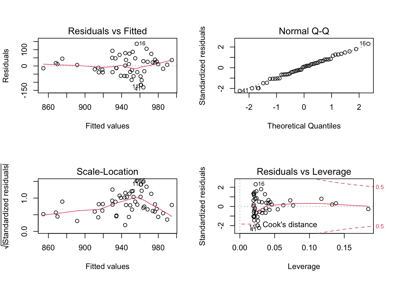
OLS regression assumptions

OLS regression relies on several assumptions, including:

The model includes all relevant variables (i.e., no omitted variable bias).
The model is linear in the parameters (i.e., the coefficients and error term).
The error term has an expected value of zero.
All right-hand-side variables are uncorrelated with the error term.
No right-hand-side variables are a perfect linear function of other RHS variables.
Observations of the error term are uncorrelated with each other.
The error term has constant variance (i.e., homoscedasticity).
(Optional - only needed for inference). The error term is normally distributed.

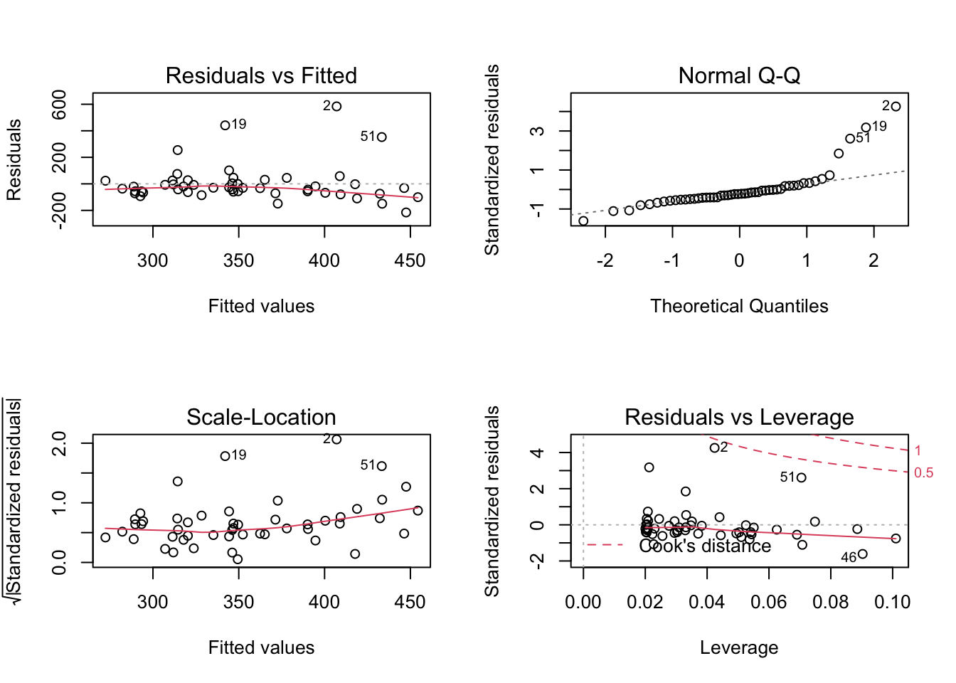
Investigate assumptions #7 and #8 visually by plotting your model:

  # split plotting area into 2 x 2 grid
  par(mfrow = c(2, 2))

  # plot model diagnostics
  plot(sat_mod)

Comparing models

Do congressional voting patterns predict SAT scores over and above expense? To find out, let’s fit two models and compare them. First, let’s create a new cleaned dataset that omits missing values in the variables we will use.

# drop missing values for the 4 variables of interest
states_voting_cleaned <- states %>%
    select(csat, expense, house, senate) %>%
    drop_na()

The drop_na() function omits rows with missing values — that is, it performs listwise deletion of observations. In some situations, we may need more flexibility. If, for example, we only want to exclude rows that have missing data for a subset of variables, we could do the following:

  # pseudocode
  df <- df %>%
    filter(!na.omit(var_name))

Now that we have a dataset with complete cases, let’s fit a more elaborate model:

  # fit another model, adding house and senate as predictors
  sat_voting_mod <- lm(csat ~ 1 + expense + house + senate,
                       data = states_voting_cleaned)

  summary(sat_voting_mod) %>% coef()

##                  Estimate   Std. Error   t value     Pr(>|t|)
## (Intercept) 1086.08037734 35.677308643 30.441769 3.964376e-32
## expense       -0.01997159  0.007781131 -2.566670 1.358758e-02
## house         -1.42370479  0.519352260 -2.741309 8.686069e-03
## senate         0.53984781  0.473469183  1.140196 2.601066e-01

To compare models, we must fit them to the same data. This is why we needed to clean the dataset. Now let’s update our first model to use these cleaned data:

  # update model using the cleaned data
  sat_mod <- sat_mod %>%
      update(data = states_voting_cleaned)

  # compare using an F-test with the anova() function
  anova(sat_mod, sat_voting_mod)

## Analysis of Variance Table
## 
## Model 1: csat ~ 1 + expense
## Model 2: csat ~ 1 + expense + house + senate
##   Res.Df    RSS Df Sum of Sq      F  Pr(>F)  
## 1     48 175049                              
## 2     46 149497  2     25552 3.9312 0.02654 *
## ---
## Signif. codes:  0 '***' 0.001 '**' 0.01 '*' 0.05 '.' 0.1 ' ' 1

Exercise 0

Ordinary least squares regression

Use the states data set. Fit a model predicting energy consumed per capita (energy) from the percentage of residents living in metropolitan areas (metro). Be sure to:

Examine/plot the data before fitting the model.

##

Print and interpret the model summary().

##

Plot the model using plot() to look for deviations from modeling assumptions.

##

Select one or more additional predictors to add to your model and repeat steps 1-3. Is this model significantly better than the model with metro as the only predictor?

##

Click for Exercise 0 Solution

Use the states data set. Fit a model predicting energy consumed per capita (energy) from the percentage of residents living in metropolitan areas (metro). Be sure to:

Examine/plot the data before fitting the model.

  states_en_met <- states %>% 
      select(energy, metro)

  summary(states_en_met)

##      energy          metro       
##  Min.   :200.0   Min.   : 20.40  
##  1st Qu.:285.0   1st Qu.: 46.98  
##  Median :320.0   Median : 67.55  
##  Mean   :354.5   Mean   : 64.07  
##  3rd Qu.:371.5   3rd Qu.: 81.58  
##  Max.   :991.0   Max.   :100.00  
##  NA's   :1       NA's   :1

  cor(states_en_met, use = "pairwise")

##            energy      metro
## energy  1.0000000 -0.3397445
## metro  -0.3397445  1.0000000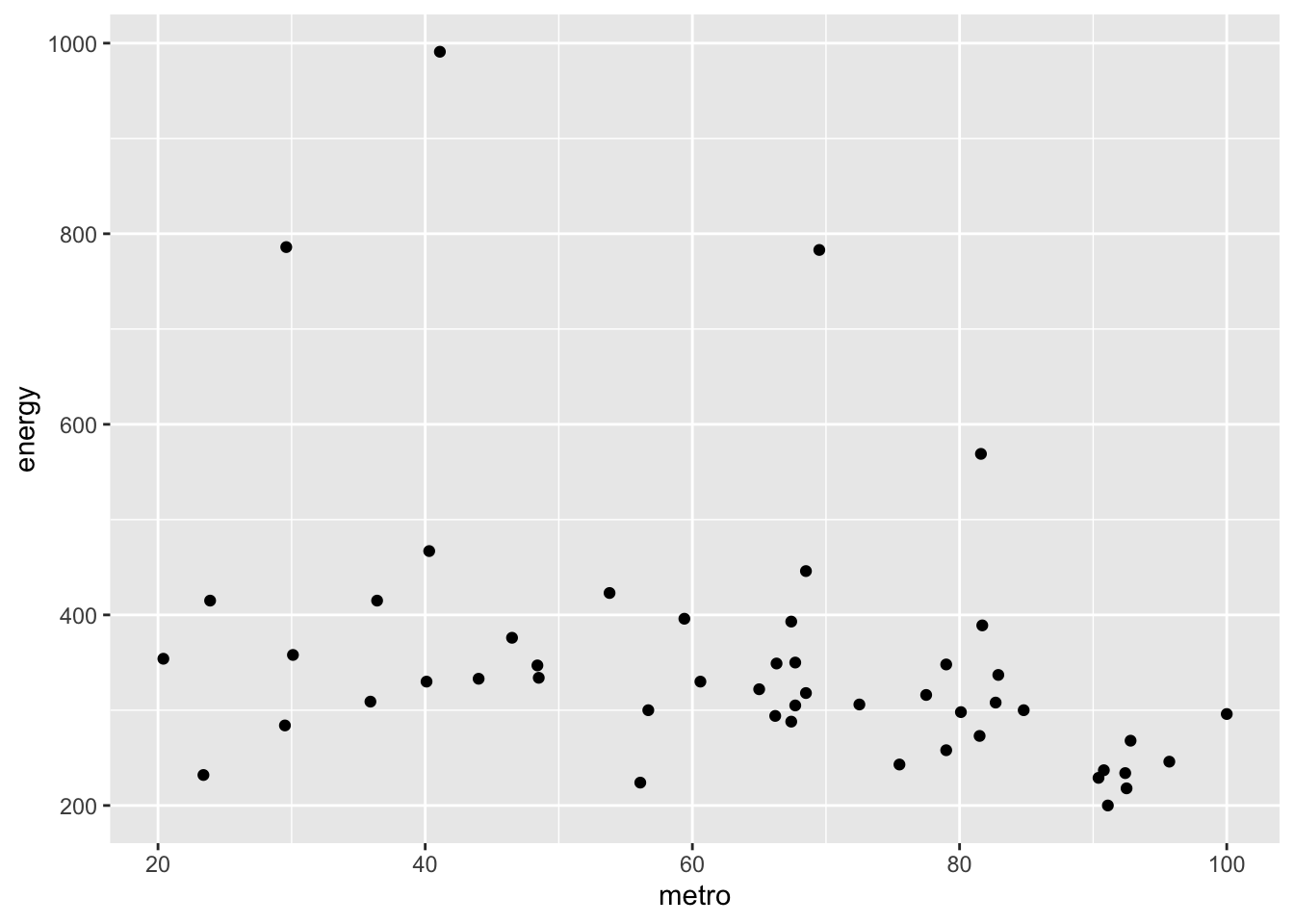

  qplot(x = metro, y = energy, geom = "point", data = states_en_met)

Print and interpret the model summary().

  mod_en_met <- lm(energy ~ metro, data = states_en_met)
  summary(mod_en_met)

## 
## Call:
## lm(formula = energy ~ metro, data = states_en_met)
## 
## Residuals:
##     Min      1Q  Median      3Q     Max 
## -215.51  -64.54  -30.87   18.71  583.97 
## 
## Coefficients:
##             Estimate Std. Error t value Pr(>|t|)    
## (Intercept) 501.0292    61.8136   8.105 1.53e-10 ***
## metro        -2.2871     0.9139  -2.503   0.0158 *  
## ---
## Signif. codes:  0 '***' 0.001 '**' 0.01 '*' 0.05 '.' 0.1 ' ' 1
## 
## Residual standard error: 140.2 on 48 degrees of freedom
##   (1 observation deleted due to missingness)
## Multiple R-squared:  0.1154, Adjusted R-squared:  0.097 
## F-statistic: 6.263 on 1 and 48 DF,  p-value: 0.01578

Plot the model using plot() to look for deviations from modeling assumptions.

  par(mfrow = c(2, 2))

  plot(mod_en_met)

Select one or more additional predictors to add to your model and repeat steps 1-3. Is this model significantly better than the model with metro as the only predictor?

  states_en_met_pop_wst <- states %>%
      select(energy, metro, pop, waste)

  summary(states_en_met_pop_wst)

##      energy          metro             pop               waste       
##  Min.   :200.0   Min.   : 20.40   Min.   :  454000   Min.   :0.5400  
##  1st Qu.:285.0   1st Qu.: 46.98   1st Qu.: 1299750   1st Qu.:0.8225  
##  Median :320.0   Median : 67.55   Median : 3390500   Median :0.9600  
##  Mean   :354.5   Mean   : 64.07   Mean   : 4962040   Mean   :0.9888  
##  3rd Qu.:371.5   3rd Qu.: 81.58   3rd Qu.: 5898000   3rd Qu.:1.1450  
##  Max.   :991.0   Max.   :100.00   Max.   :29760000   Max.   :1.5100  
##  NA's   :1       NA's   :1        NA's   :1          NA's   :1

  cor(states_en_met_pop_wst, use = "pairwise")

##            energy      metro        pop      waste
## energy  1.0000000 -0.3397445 -0.1840357 -0.2526499
## metro  -0.3397445  1.0000000  0.5653562  0.4877881
## pop    -0.1840357  0.5653562  1.0000000  0.5255713
## waste  -0.2526499  0.4877881  0.5255713  1.0000000

  mod_en_met_pop_waste <- lm(energy ~ 1 + metro + pop + waste, data = states_en_met_pop_wst)
  summary(mod_en_met_pop_waste)

## 
## Call:
## lm(formula = energy ~ 1 + metro + pop + waste, data = states_en_met_pop_wst)
## 
## Residuals:
##     Min      1Q  Median      3Q     Max 
## -224.62  -67.48  -31.76   12.65  589.48 
## 
## Coefficients:
##               Estimate Std. Error t value Pr(>|t|)    
## (Intercept)  5.617e+02  9.905e+01   5.671    9e-07 ***
## metro       -2.079e+00  1.168e+00  -1.780   0.0816 .  
## pop          1.649e-06  4.809e-06   0.343   0.7332    
## waste       -8.307e+01  1.042e+02  -0.797   0.4295    
## ---
## Signif. codes:  0 '***' 0.001 '**' 0.01 '*' 0.05 '.' 0.1 ' ' 1
## 
## Residual standard error: 142.2 on 46 degrees of freedom
##   (1 observation deleted due to missingness)
## Multiple R-squared:  0.1276, Adjusted R-squared:  0.07067 
## F-statistic: 2.242 on 3 and 46 DF,  p-value: 0.09599

  anova(mod_en_met, mod_en_met_pop_waste)

## Analysis of Variance Table
## 
## Model 1: energy ~ metro
## Model 2: energy ~ 1 + metro + pop + waste
##   Res.Df    RSS Df Sum of Sq      F Pr(>F)
## 1     48 943103                           
## 2     46 930153  2     12949 0.3202 0.7276

Interactions & factors

GOAL: To learn how to specify interaction effects and fit models with categorical predictors. In particular:

Formula syntax for interaction effects
Factor levels and labels
Contrasts and pairwise comparisons

Modeling interactions

Interactions allow us assess the extent to which the association between one predictor and the outcome depends on a second predictor. For example: does the association between expense and SAT scores depend on the median income in the state?

  # add the interaction to a model
  sat_expense_by_income <- lm(csat ~ 1 + expense + income + expense : income, data = states)

  # same as above, but shorter syntax
  sat_expense_by_income <- lm(csat ~ 1 + expense * income, data = states) 

  # show the regression coefficients table
  summary(sat_expense_by_income) %>% coef()

##                     Estimate   Std. Error   t value     Pr(>|t|)
## (Intercept)     1.380364e+03 1.720863e+02  8.021351 2.367069e-10
## expense        -6.384067e-02 3.270087e-02 -1.952262 5.687837e-02
## income         -1.049785e+01 4.991463e+00 -2.103161 4.083253e-02
## expense:income  1.384647e-03 8.635529e-04  1.603431 1.155395e-01

Regression with categorical predictors

Let’s try to predict SAT scores (csat) from geographical region (region), a categorical variable. Note that you must make sure R does not think your categorical variable is numeric.

  # make sure R knows region is categorical
  str(states$region)

##  Factor w/ 4 levels "West","N. East",..: 3 1 1 3 1 1 2 3 NA 3 ...

Here, R is already treating region as categorical — that is, in R parlance, a “factor” variable. If region were not already a factor, we could make it so like this:

  # convert `region` to a factor
  states <- states %>%
      mutate(region = factor(region))

  # arguments to the factor() function:
  # factor(x, levels, labels)

  # examine factor levels
  levels(states$region)

## [1] "West"    "N. East" "South"   "Midwest"

Now let’s add region to the model:

  # add region to the model
  sat_region <- lm(csat ~ 1 + region, data = states) 

  # show the results
  summary(sat_region) %>% coef() # show only the regression coefficients table

##                Estimate Std. Error    t value     Pr(>|t|)
## (Intercept)   946.30769   14.79582 63.9577807 1.352577e-46
## regionN. East -56.75214   23.13285 -2.4533141 1.800383e-02
## regionSouth   -16.30769   19.91948 -0.8186806 4.171898e-01
## regionMidwest  63.77564   21.35592  2.9863209 4.514152e-03

We can get an omnibus F-test for region by using the anova() method:

  anova(sat_region) # show ANOVA table

## Analysis of Variance Table
## 
## Response: csat
##           Df Sum Sq Mean Sq F value    Pr(>F)    
## region     3  82049 27349.8  9.6102 4.859e-05 ***
## Residuals 46 130912  2845.9                      
## ---
## Signif. codes:  0 '***' 0.001 '**' 0.01 '*' 0.05 '.' 0.1 ' ' 1

So, make sure to tell R which variables are categorical by converting them to factors!

Setting factor reference groups & contrasts

Contrasts is the umbrella term used to describe the process of testing linear combinations of parameters from regression models. All statistical sofware use contrasts, but each software has different defaults and their own way of overriding these.

The default contrasts in R are “treatment” contrasts (aka “dummy coding”), where each level within a factor is identified within a matrix of binary 0 / 1 variables, with the first level chosen as the reference category. They’re called “treatment” contrasts, because of the typical use case where there is one control group (the reference group) and one or more treatment groups that are to be compared to the controls. It is easy to change the default contrasts to something other than treatment contrasts, though this is rarely needed. More often, we may want to change the reference group in treatment contrasts or get all sets of pairwise contrasts between factor levels.

First, let’s examine the default contrasts for region:

  # default treatment (dummy) contrasts
  contrasts(states$region)

##         N. East South Midwest
## West          0     0       0
## N. East       1     0       0
## South         0     1       0
## Midwest       0     0       1

We can see that the reference level is West. How can we change this? Let’s use the relevel() function:

  # change the reference group
  states <- states %>%
      mutate(region = relevel(region, ref = "Midwest"))

  # check the reference group has changed
  contrasts(states$region)

##         West N. East South
## Midwest    0       0     0
## West       1       0     0
## N. East    0       1     0
## South      0       0     1

Now the reference level has changed to Midwest. Let’s refit the model with the releveled region variable:

  # refit the model
  mod_region <- lm(csat ~ 1 + region, data = states)

  # print summary coefficients table
  summary(mod_region) %>% coef()

##                 Estimate Std. Error   t value     Pr(>|t|)
## (Intercept)   1010.08333   15.39998 65.589930 4.296307e-47
## regionWest     -63.77564   21.35592 -2.986321 4.514152e-03
## regionN. East -120.52778   23.52385 -5.123641 5.798399e-06
## regionSouth    -80.08333   20.37225 -3.931000 2.826007e-04

Often, we may want to get all possible pairwise comparisons among the various levels of a factor variable, rather than just compare particular levels to a single reference level. We could of course just keep changing the reference level and refitting the model, but this would be tedious. Instead, we can use the emmeans() post-estimation function from the emmeans package to do the calculations for us:

  # get all pairwise contrasts between means
  mod_region %>%
      emmeans(specs = pairwise ~ region)

## $emmeans
##  region  emmean   SE df lower.CL upper.CL
##  Midwest   1010 15.4 46      979     1041
##  West       946 14.8 46      917      976
##  N. East    890 17.8 46      854      925
##  South      930 13.3 46      903      957
## 
## Confidence level used: 0.95 
## 
## $contrasts
##  contrast          estimate   SE df t.ratio p.value
##  Midwest - West        63.8 21.4 46  2.986  0.0226 
##  Midwest - N. East    120.5 23.5 46  5.124  <.0001 
##  Midwest - South       80.1 20.4 46  3.931  0.0016 
##  West - N. East        56.8 23.1 46  2.453  0.0812 
##  West - South          16.3 19.9 46  0.819  0.8453 
##  N. East - South      -40.4 22.2 46 -1.820  0.2774 
## 
## P value adjustment: tukey method for comparing a family of 4 estimates

Exercise 1

Interactions & factors

Use the states data set.

Add on to the regression equation that you created in Exercise 1 by generating an interaction term and testing the interaction.

##

Try adding region to the model. Are there significant differences across the four regions?

##

Click for Exercise 1 Solution

Use the states data set.

Add on to the regression equation that you created in exercise 1 by generating an interaction term and testing the interaction.

  mod_en_metro_by_waste <- lm(energy ~ 1 + metro * waste, data = states)

Try adding region to the model. Are there significant differences across the four regions?

  mod_en_region <- lm(energy ~ 1 + metro * waste + region, data = states)
  anova(mod_en_metro_by_waste, mod_en_region)

## Analysis of Variance Table
## 
## Model 1: energy ~ 1 + metro * waste
## Model 2: energy ~ 1 + metro * waste + region
##   Res.Df    RSS Df Sum of Sq    F Pr(>F)
## 1     46 930683                         
## 2     43 821247  3    109436 1.91 0.1422

Models with binary outcomes

GOAL: To learn how to use the glm() function to model binary outcomes. In particular:

The family and link components of the glm() function call
Transforming model coefficients into odds ratios
Transforming model coefficients into predicted marginal means

Logistic regression

Thus far we have used the lm() function to fit our regression models. lm() is great, but limited — in particular it only fits models for continuous dependent variables. For categorical dependent variables we can use the glm() function.

For these models we will use a different dataset, drawn from the National Health Interview Survey. From the CDC website:

The National Health Interview Survey (NHIS) has monitored the health of the nation since 1957. NHIS data on a broad range of health topics are collected through personal household interviews. For over 50 years, the U.S. Census Bureau has been the data collection agent for the National Health Interview Survey. Survey results have been instrumental in providing data to track health status, health care access, and progress toward achieving national health objectives.

Load the National Health Interview Survey data:

  NH11 <- read_rds("dataSets/NatHealth2011.rds")

Logistic regression example

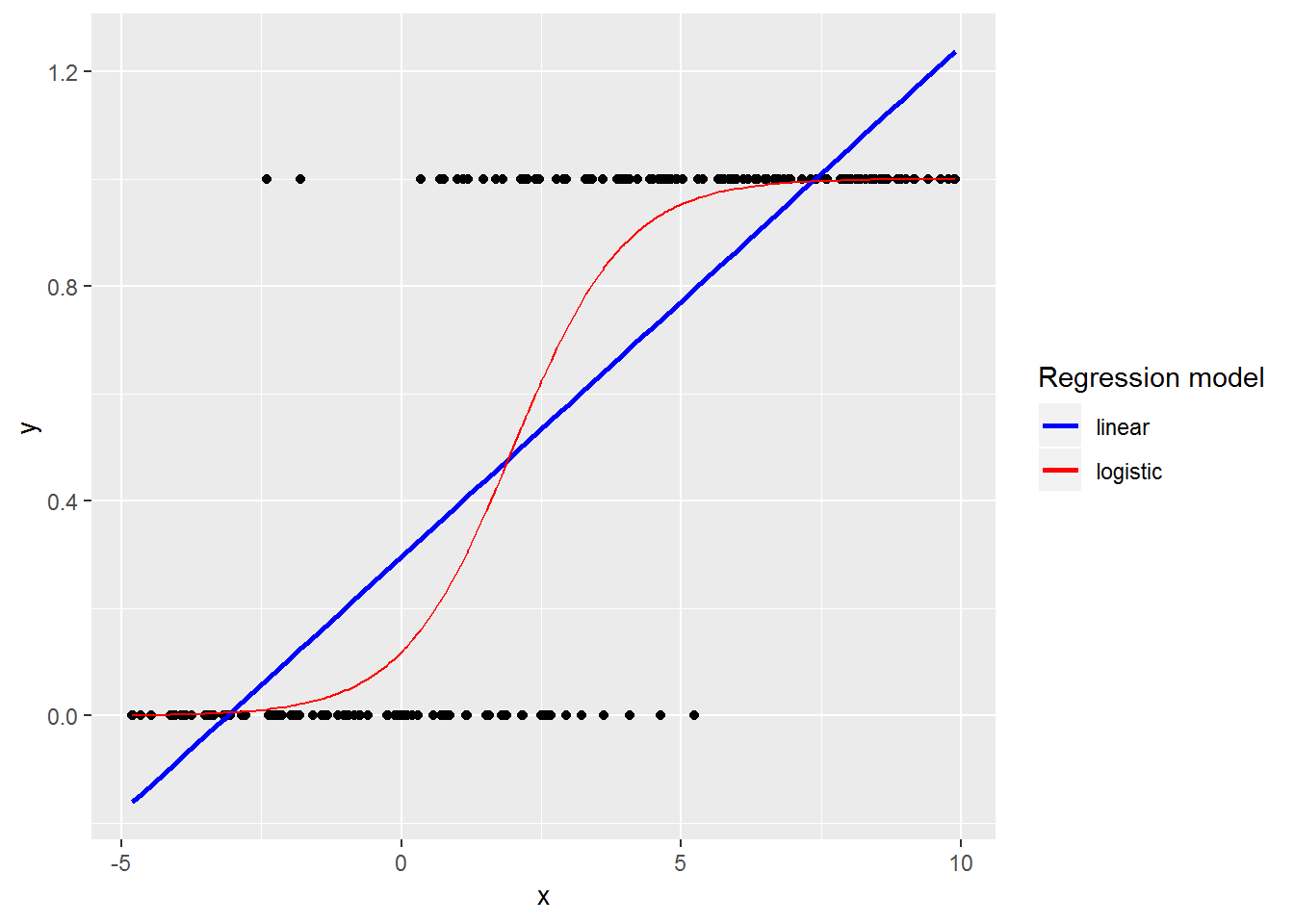
If we were to use a linear model, rather than a logistic model, when we have a binary response we would find that:

Explanatory variables will not be linearly related to the outcome
Residuals will not be normally distributed
Variance will not be homoskedastic
Predictions will not be constrained to be on the interval [0, 1]

Though, some of these issues can be dealt with by estimating a linear probability model with robust standard errors.

Anatomy of a generalized linear model:

  # OLS model using lm()
  lm(outcome ~ 1 + pred1 + pred2, 
     data = mydata)

  # OLS model using glm()
  glm(outcome ~ 1 + pred1 + pred2, 
      data = mydata, 
      family = gaussian(link = "identity"))
 
  # logistic model using glm()
  glm(outcome ~ 1 + pred1 + pred2, 
      data = mydata, 
      family = binomial(link = "logit"))

The family argument sets the error distribution for the model, while the link function argument relates the predictors to the expected value of the outcome.

Let’s predict the probability of being diagnosed with hypertension based on age, sex, sleep, and bmi. Here’s the theoretical model:

\[ logit(p(hypertension_i = 1)) = \beta_{0}1 + \beta_1age_i + \beta_2sex_i + \beta_3sleep_i + \beta_4bmi_i \]

where $logit(\cdot)$ is the non-linear link function that relates a linear expression of the predictors to the expectation of the binary response:

\[ logit(p(hypertension_i = 1)) = ln \left( \frac{p(hypertension_i = 1)}{1-p(hypertension_i = 1)} \right) = ln \left( \frac{p(hypertension_i = 1)}{p(hypertension_i = 0)} \right) \]

And here’s how we fit this model in R. First, let’s clean up the hypertension outcome by making it binary:

  str(NH11$hypev) # check stucture of hypev

##  Factor w/ 5 levels "1 Yes","2 No",..: 2 2 1 2 2 1 2 2 1 2 ...

  levels(NH11$hypev) # check levels of hypev

## [1] "1 Yes"             "2 No"              "7 Refused"        
## [4] "8 Not ascertained" "9 Don't know"

  # collapse all missing values to NA
  NH11 <- NH11 %>%
      mutate(hypev = factor(hypev, levels=c("2 No", "1 Yes")))

Now let’s use glm() to estimate the model:

  # run our regression model
  hyp_out <- glm(hypev ~ 1 + age_p + sex + sleep + bmi,
                 data = NH11, 
                 family = binomial(link = "logit"))
  
  # summary model coefficients table
  summary(hyp_out) %>% coef()

##                 Estimate   Std. Error    z value     Pr(>|z|)
## (Intercept) -4.269466028 0.0564947294 -75.572820 0.000000e+00
## age_p        0.060699303 0.0008227207  73.778743 0.000000e+00
## sex2 Female -0.144025092 0.0267976605  -5.374540 7.677854e-08
## sleep       -0.007035776 0.0016397197  -4.290841 1.779981e-05
## bmi          0.018571704 0.0009510828  19.526906 6.485172e-85

Odds ratios

Generalized linear models use link functions to relate the average value of the response to the predictors, so raw coefficients are difficult to interpret. For example, the age coefficient of 0.06 in the previous model tells us that for every one unit increase in age, the log odds of hypertension diagnosis increases by 0.06. Since most of us are not used to thinking in log odds this is not too helpful!

One solution is to transform the coefficients to make them easier to interpret. Here we transform them into odds ratios by exponentiating:

  # point estimates
  coef(hyp_out) %>% exp()

## (Intercept)       age_p sex2 Female       sleep         bmi 
##  0.01398925  1.06257935  0.86586602  0.99298892  1.01874523

  # confidence intervals
  confint(hyp_out) %>% exp()

##                  2.5 %     97.5 %
## (Intercept) 0.01251677 0.01561971
## age_p       1.06087385 1.06430082
## sex2 Female 0.82155196 0.91255008
## sleep       0.98978755 0.99617465
## bmi         1.01685145 1.02065009

Predicted marginal means

Instead of reporting odds ratios, we may want to calculate predicted marginal means (sometimes called “least-squares means” or “estimated marginal means”). These are average values of the outcome at particular levels of the predictors. For ease of interpretation, we want these marginal means to be on the response scale (i.e., the probability scale). We can use the effects package to compute these quantities of interest for us (by default, the numerical output will be on the response scale).

  # get predicted marginal means
  hyp_out %>% 
      allEffects() %>%
      plot(type = "response") # "response" refers to the probability scale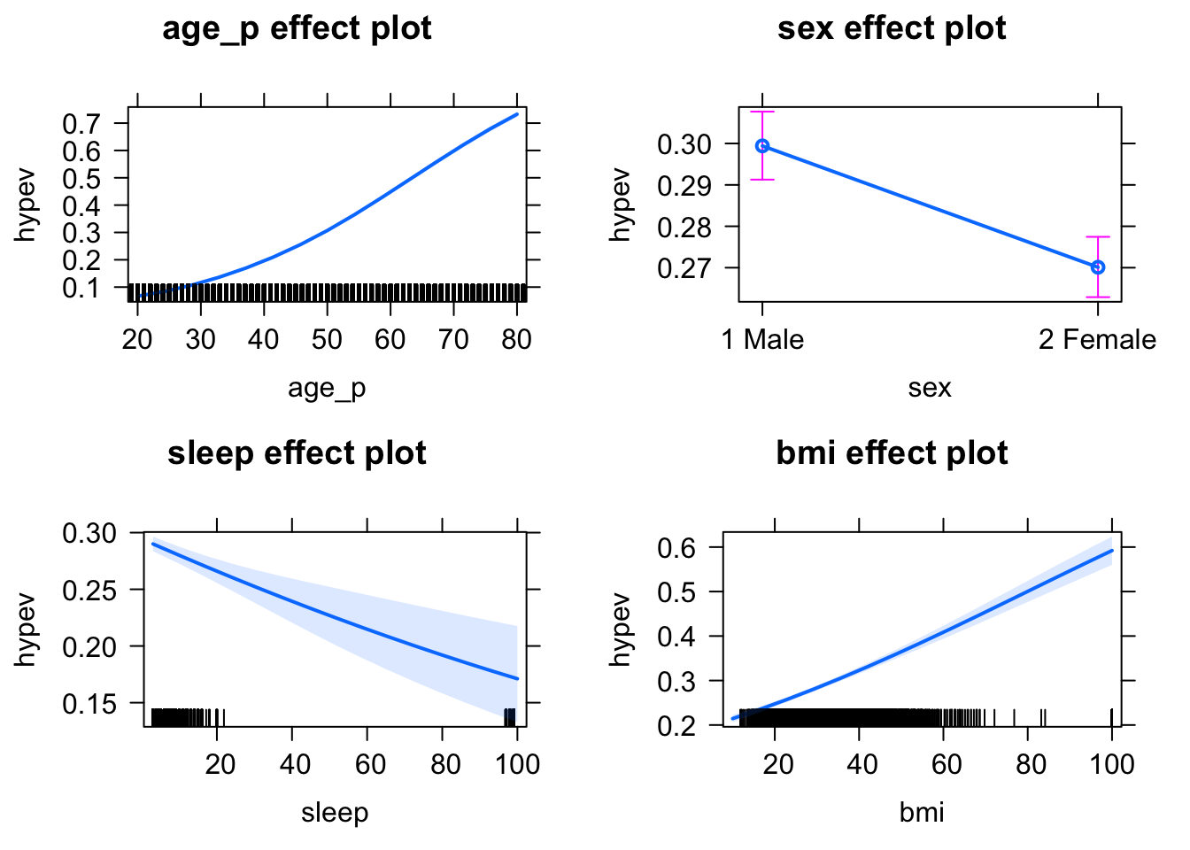

By default, allEffects() will produce predictions for all levels of factor variables, while for continuous variables it will chose 5 representative values based on quantiles. We can easily override this behavior using the xlevels argument and get predictions at any values of a continuous variable.

  # generate a sequence of ages at which to get predictions of the outcome
  age_years <- seq(20, 80, by = 5)
  age_years

##  [1] 20 25 30 35 40 45 50 55 60 65 70 75 80

  # get predicted marginal means
  eff_df <- 
      hyp_out %>% 
      allEffects(xlevels = list(age_p = age_years)) %>% # override defaults for age
      as.data.frame() # get confidence intervals
  
  eff_df

## $age_p
##    age_p        fit          se      lower      upper
## 1     20 0.06690384 0.001915704 0.06324553 0.07075778
## 2     25 0.08852692 0.002181618 0.08434323 0.09289708
## 3     30 0.11626770 0.002418813 0.11161020 0.12109307
## 4     35 0.15125876 0.002603243 0.14622690 0.15643204
## 5     40 0.19446321 0.002722428 0.18918282 0.19985467
## 6     45 0.24642528 0.002796260 0.24098582 0.25194677
## 7     50 0.30698073 0.002895857 0.30133437 0.31268554
## 8     55 0.37501156 0.003124112 0.36890868 0.38115441
## 9     60 0.44836479 0.003531792 0.44145305 0.45529654
## 10    65 0.52403564 0.004052454 0.51608756 0.53197156
## 11    70 0.59861876 0.004545531 0.58967801 0.60749436
## 12    75 0.66889903 0.004880732 0.65926418 0.67839434
## 13    80 0.73237506 0.004986539 0.72248912 0.74203457
## 
## $sex
##        sex       fit          se     lower     upper
## 1   1 Male 0.2994186 0.004188707 0.2912739 0.3076922
## 2 2 Female 0.2701044 0.003715028 0.2628852 0.2774472
## 
## $sleep
##   sleep       fit          se     lower     upper
## 1     3 0.2899941 0.003276427 0.2836147 0.2964575
## 2    30 0.2524895 0.007427001 0.2382124 0.2673219
## 3    50 0.2268657 0.012446183 0.2034008 0.2521806
## 4    80 0.1919843 0.018549461 0.1582199 0.2309771
## 5   100 0.1710955 0.021584286 0.1328287 0.2176200
## 
## $bmi
##   bmi       fit          se     lower     upper
## 1  10 0.2144084 0.004121590 0.2064409 0.2225972
## 2  30 0.2835093 0.002849407 0.2779580 0.2891272
## 3  60 0.4085485 0.007450161 0.3940311 0.4232272
## 4  80 0.5003663 0.012139141 0.4765911 0.5241398
## 5 100 0.5921593 0.016180071 0.5601051 0.6234481

Exercise 2

Logistic regression

Use the NH11 data set that we loaded earlier. Note that the data are not perfectly clean and ready to be modeled. You will need to clean up at least some of the variables before fitting the model.

Use glm() to conduct a logistic regression to predict ever worked (everwrk) using age (age_p) and marital status (r_maritl). Make sure you only keep the following two levels for everwrk (2 No and 1 Yes). Hint: use the factor() function. Also, make sure to drop any r_maritl levels that do not contain observations. Hint: see ?droplevels.

##

Predict the probability of working for each level of marital status. Hint: use allEffects()

##

Note that the data are not perfectly clean and ready to be modeled. You will need to clean up at least some of the variables before fitting the model.

Click for Exercise 2 Solution

Use the NH11 data set that we loaded earlier. Note that the data are not perfectly clean and ready to be modeled. You will need to clean up at least some of the variables before fitting the model.

Use glm() to conduct a logistic regression to predict ever worked (everwrk) using age (age_p) and marital status (r_maritl). Make sure you only keep the following two levels for everwrk (2 No and 1 Yes). Hint: use the factor() function. Also, make sure to drop any r_maritl levels that do not contain observations. Hint: see ?droplevels.

  NH11 <- NH11 %>%
      mutate(everwrk = factor(everwrk, levels = c("2 No", "1 Yes")),
             r_maritl = droplevels(r_maritl)
             )

  mod_wk_age_mar <- glm(everwrk ~ 1 + age_p + r_maritl, 
                        data = NH11,
                        family = binomial(link = "logit"))

  summary(mod_wk_age_mar)

## 
## Call:
## glm(formula = everwrk ~ 1 + age_p + r_maritl, family = binomial(link = "logit"), 
##     data = NH11)
## 
## Deviance Residuals: 
##     Min       1Q   Median       3Q      Max  
## -2.7308   0.3370   0.4391   0.5650   1.0436  
## 
## Coefficients:
##                                              Estimate Std. Error z value
## (Intercept)                                  0.440248   0.093538   4.707
## age_p                                        0.029812   0.001645  18.118
## r_maritl2 Married - spouse not in household -0.049675   0.217310  -0.229
## r_maritl4 Widowed                           -0.683618   0.084335  -8.106
## r_maritl5 Divorced                           0.730115   0.111681   6.538
## r_maritl6 Separated                          0.128091   0.151366   0.846
## r_maritl7 Never married                     -0.343611   0.069222  -4.964
## r_maritl8 Living with partner                0.443583   0.137770   3.220
## r_maritl9 Unknown marital status            -0.395480   0.492967  -0.802
##                                             Pr(>|z|)    
## (Intercept)                                 2.52e-06 ***
## age_p                                        < 2e-16 ***
## r_maritl2 Married - spouse not in household  0.81919    
## r_maritl4 Widowed                           5.23e-16 ***
## r_maritl5 Divorced                          6.25e-11 ***
## r_maritl6 Separated                          0.39742    
## r_maritl7 Never married                     6.91e-07 ***
## r_maritl8 Living with partner                0.00128 ** 
## r_maritl9 Unknown marital status             0.42241    
## ---
## Signif. codes:  0 '***' 0.001 '**' 0.01 '*' 0.05 '.' 0.1 ' ' 1
## 
## (Dispersion parameter for binomial family taken to be 1)
## 
##     Null deviance: 11082  on 14039  degrees of freedom
## Residual deviance: 10309  on 14031  degrees of freedom
##   (18974 observations deleted due to missingness)
## AIC: 10327
## 
## Number of Fisher Scoring iterations: 5

Predict the probability of working for each level of marital status. Hint: use allEffects().

  mod_wk_age_mar %>% 
      allEffects() %>%
      as.data.frame()

## $age_p
##   age_p       fit          se     lower     upper
## 1    20 0.7241256 0.011448539 0.7011322 0.7459909
## 2    30 0.7795664 0.007483648 0.7645495 0.7938837
## 3    50 0.8652253 0.003183752 0.8588624 0.8713443
## 4    70 0.9209721 0.003053617 0.9147761 0.9267537
## 5    80 0.9401248 0.003123927 0.9337009 0.9459624
## 
## $r_maritl
##                              r_maritl       fit          se     lower     upper
## 1     1 Married - spouse in household 0.8917800 0.004259644 0.8831439 0.8998502
## 2 2 Married - spouse not in household 0.8868918 0.021393167 0.8377247 0.9225394
## 3                           4 Widowed 0.8061891 0.010634762 0.7844913 0.8261864
## 4                          5 Divorced 0.9447561 0.005361664 0.9332564 0.9543712
## 5                         6 Separated 0.9035358 0.012707502 0.8755978 0.9257318
## 6                     7 Never married 0.8538900 0.007459212 0.8386559 0.8679122
## 7               8 Living with partner 0.9277504 0.008904955 0.9082334 0.9433753
## 8            9 Unknown marital status 0.8472992 0.063528455 0.6794427 0.9355916

Multilevel modeling

GOAL: To learn about how to use the lmer() function to model clustered data. In particular:

The formula syntax for incorporating random effects into a model
Calculating the intraclass correlation (ICC)
Model comparison for fixed and random effects

Multilevel modeling overview

Multi-level (AKA hierarchical) models are a type of mixed-effects model
They are used to model data that are clustered (i.e., non-independent)
Mixed-effects models include two types of predictors: fixed-effects and random effects
- Fixed-effects – observed levels are of direct interest (.e.g, sex, political party…)
- Random-effects – observed levels not of direct interest: goal is to make inferences to a population represented by observed levels
- In R, the lme4 package is the most popular for mixed effects models
- Use the lmer() function for linear mixed models, glmer() for generalized linear mixed models

The Exam data

The Exam.rds data set contains exam scores of 4,059 students from 65 schools in Inner London. The variable names are as follows:

Variable	Description
school	School ID - a factor.
normexam	Normalized exam score.
standLRT	Standardized LR test score.
student	Student id (within school) - a factor

Let’s read in the data:

  exam <- read_rds("dataSets/Exam.rds")

The null model & ICC

Before we fit our first model, let’s take a look at the R syntax for multilevel models:

  # anatomy of lmer() function
  lmer(outcome ~ 1 + pred1 + pred2 + (1 | grouping_variable), 
       data = mydata)

Notice the formula section within the brackets: (1 | grouping_variable). This part of the formula tells R about the hierarchical structure of the model. In this case, it says we have a model with random intercepts (1) grouped by (|) a grouping_variable.

As a preliminary modeling step, it is often useful to partition the variance in the dependent variable into the various levels. This can be accomplished by running a null model (i.e., a model with a random effects grouping structure, but no fixed-effects predictors) and then calculating the intra-class correlation (ICC).

  # null model, grouping by school but not fixed effects.
  Norm1 <-lmer(normexam ~ 1 + (1 | school), 
               data = na.omit(exam))
  summary(Norm1)

## Linear mixed model fit by REML ['lmerMod']
## Formula: normexam ~ 1 + (1 | school)
##    Data: na.omit(exam)
## 
## REML criterion at convergence: 9962.9
## 
## Scaled residuals: 
##     Min      1Q  Median      3Q     Max 
## -3.8749 -0.6452  0.0045  0.6888  3.6836 
## 
## Random effects:
##  Groups   Name        Variance Std.Dev.
##  school   (Intercept) 0.1634   0.4042  
##  Residual             0.8520   0.9231  
## Number of obs: 3662, groups:  school, 65
## 
## Fixed effects:
##             Estimate Std. Error t value
## (Intercept) -0.01310    0.05312  -0.247

The ICC is calculated as .163/(.163 + .852) = .161, which means that ~16% of the variance is at the school level.

There is no consensus on how to calculate p-values for MLMs; hence why they are omitted from the lme4 output. But, if you really need p-values, the lmerTest package will calculate p-values for you (using the Satterthwaite approximation).

Adding fixed-effects predictors

Here’s a theoretical model that predicts exam scores from student’s standardized tests scores:

\[ examscores_{ij} = \mu1 + \beta_1testscores_{ij} + U_{0j} + \epsilon_{ij} \]

where $U_{0j}$ is the random intercept for the $j$^th school. Let’s implement this in R using lmer():

  # model with exam scores regressed on student's standardized tests scores
  Norm2 <-lmer(normexam ~ 1 + standLRT + (1 | school),
               data = na.omit(exam)) 
  summary(Norm2)

## Linear mixed model fit by REML ['lmerMod']
## Formula: normexam ~ 1 + standLRT + (1 | school)
##    Data: na.omit(exam)
## 
## REML criterion at convergence: 8483.5
## 
## Scaled residuals: 
##     Min      1Q  Median      3Q     Max 
## -3.6725 -0.6300  0.0234  0.6777  3.3340 
## 
## Random effects:
##  Groups   Name        Variance Std.Dev.
##  school   (Intercept) 0.09369  0.3061  
##  Residual             0.56924  0.7545  
## Number of obs: 3662, groups:  school, 65
## 
## Fixed effects:
##               Estimate Std. Error t value
## (Intercept) -4.313e-05  4.055e-02  -0.001
## standLRT     5.669e-01  1.324e-02  42.821
## 
## Correlation of Fixed Effects:
##          (Intr)
## standLRT 0.007

Multiple degree of freedom comparisons

As with lm() and glm() models, you can compare the two lmer() models using the anova() function. With mixed effects models, this will produce a likelihood ratio test.

  # likelihood ratio test of two nested models
  anova(Norm1, Norm2)

## Data: na.omit(exam)
## Models:
## Norm1: normexam ~ 1 + (1 | school)
## Norm2: normexam ~ 1 + standLRT + (1 | school)
##       npar    AIC    BIC  logLik deviance  Chisq Df Pr(>Chisq)    
## Norm1    3 9964.9 9983.5 -4979.4   9958.9                         
## Norm2    4 8480.1 8505.0 -4236.1   8472.1 1486.8  1  < 2.2e-16 ***
## ---
## Signif. codes:  0 '***' 0.001 '**' 0.01 '*' 0.05 '.' 0.1 ' ' 1

Random slopes

We can add a random effect of students’ standardized test scores as well. Now in addition to estimating the distribution of intercepts across schools, we also estimate the distribution of the slope of exam on standardized test.

  # add random effect of students' standardized test scores to model
  Norm3 <- lmer(normexam ~ 1 + standLRT + (1 + standLRT | school), 
                data = na.omit(exam)) 
  summary(Norm3)

## Linear mixed model fit by REML ['lmerMod']
## Formula: normexam ~ 1 + standLRT + (1 + standLRT | school)
##    Data: na.omit(exam)
## 
## REML criterion at convergence: 8442.8
## 
## Scaled residuals: 
##     Min      1Q  Median      3Q     Max 
## -3.7904 -0.6246  0.0245  0.6734  3.4376 
## 
## Random effects:
##  Groups   Name        Variance Std.Dev. Corr
##  school   (Intercept) 0.09092  0.3015       
##           standLRT    0.01639  0.1280   0.49
##  Residual             0.55589  0.7456       
## Number of obs: 3662, groups:  school, 65
## 
## Fixed effects:
##             Estimate Std. Error t value
## (Intercept) -0.01250    0.04011  -0.312
## standLRT     0.56094    0.02119  26.474
## 
## Correlation of Fixed Effects:
##          (Intr)
## standLRT 0.360

Test the significance of the random slope

To test the significance of a random slope just compare models with and without the random slope term using a likelihood ratio test:

  # likelihood ratio test for random slope term
  anova(Norm2, Norm3)

## Data: na.omit(exam)
## Models:
## Norm2: normexam ~ 1 + standLRT + (1 | school)
## Norm3: normexam ~ 1 + standLRT + (1 + standLRT | school)
##       npar    AIC    BIC  logLik deviance Chisq Df Pr(>Chisq)    
## Norm2    4 8480.1 8505.0 -4236.1   8472.1                        
## Norm3    6 8444.1 8481.4 -4216.1   8432.1 40.01  2  2.051e-09 ***
## ---
## Signif. codes:  0 '***' 0.001 '**' 0.01 '*' 0.05 '.' 0.1 ' ' 1

Exercise 3

Multilevel modeling

Use the bh1996 dataset:

## install.packages("multilevel")
data(bh1996, package = "multilevel")

From the data documentation:

Variables are Leadership Climate (LEAD), Well-Being (WBEING), and Work Hours (HRS). The group identifier is named GRP.

Create a null model predicting wellbeing (WBEING)

##

Calculate the ICC for your null model

##

Run a second multi-level model that adds two individual-level predictors, average number of hours worked (HRS) and leadership skills (LEAD) to the model and interpret your output.

##

Now, add a random effect of average number of hours worked (HRS) to the model and interpret your output. Test the significance of this random term.

##

Click for Exercise 3 Solution

Use the dataset bh1996:

  # install.packages("multilevel")
  data(bh1996, package="multilevel")