Suggested Programming Solutions
library(dplyr)
library(readr)
library(ggplot2)
library(ggrepel)
library(forcats)
library(scales)
15.5 Chapter 10: Visualization
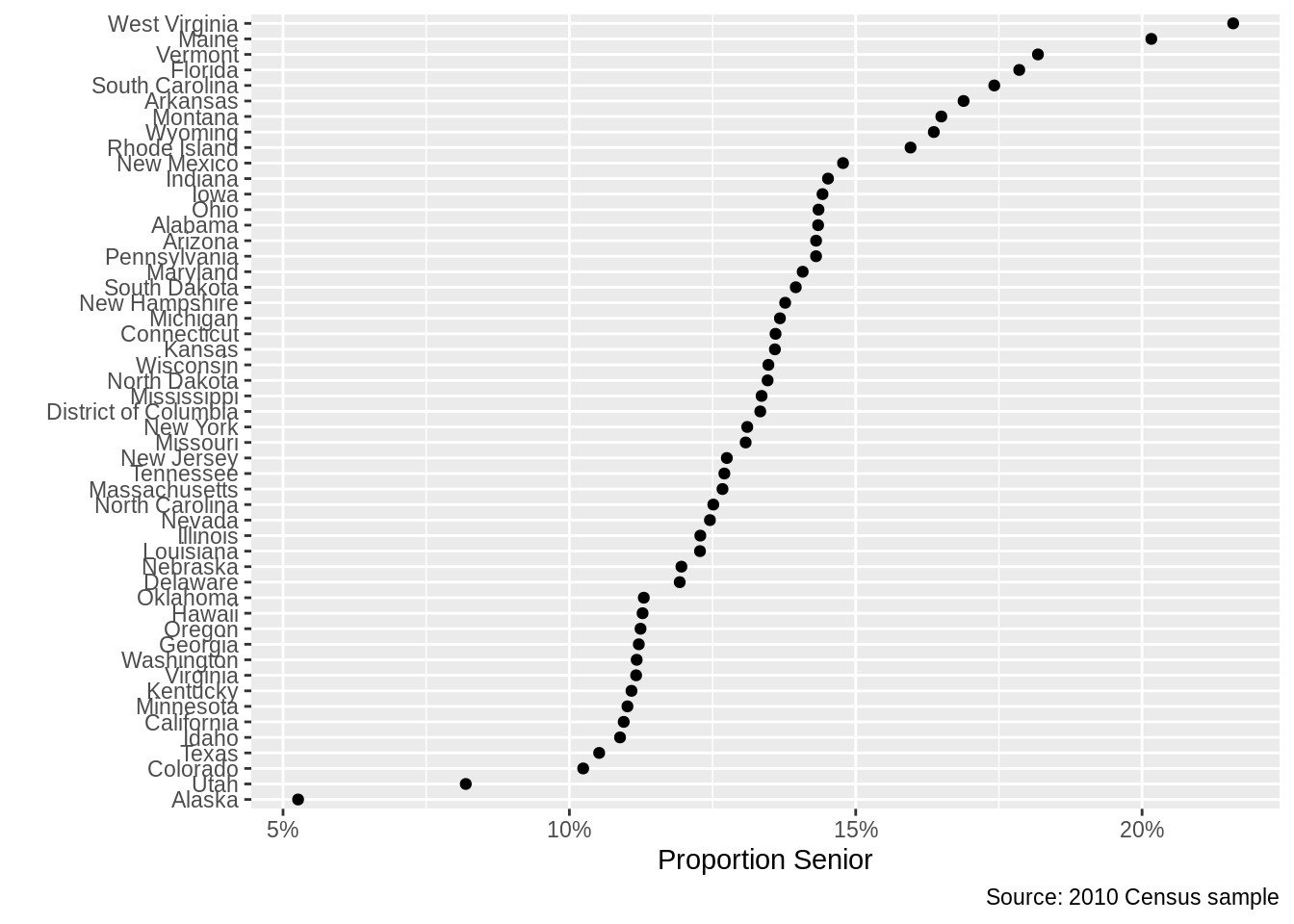
1 State Proportions
cen10 <- readRDS("data/input/usc2010_001percent.Rds")Group by state, noting that the mean of a set of logicals is a mean of 1s (TRUE) and 0s (FALSE).
grp_st <- cen10 %>%
  group_by(state) %>%
  summarize(prop = mean(age >= 65)) %>%
  arrange(prop) %>%
  mutate(state = as_factor(state))
## `summarise()` ungrouping output (override with `.groups` argument)Plot points
ggplot(grp_st, aes(x = state, y = prop)) +
  geom_point() +
  coord_flip() +
  scale_y_continuous(labels = percent_format(accuracy = 1)) + # use the scales package to format percentages
  labs(
    y = "Proportion Senior",
    x = "",
    caption = "Source: 2010 Census sample"
  )
2 Swing Justice
justices <- read_csv("data/input/justices_court-median.csv")Keep justices who are in the dataset in 2016,
in_2017 <- justices %>%
  filter(term >= 2016) %>%
  distinct(justice) %>% # unique values
  mutate(present_2016 = 1) # keep an indicator to distinguish from rest after merge

df_indicator <- justices %>%
  left_join(in_2017)
## Joining, by = "justice"All together
ggplot(df_indicator, aes(x = term, y = idealpt, group = justice_id)) +
  geom_line(aes(y = median_idealpt), color = "red", size = 2, alpha = 0.1) +
  geom_line(alpha = 0.5) +
  geom_line(data = filter(df_indicator, !is.na(present_2016))) +
  geom_point(data = filter(df_indicator, !is.na(present_2016), term == 2018)) +
  geom_text_repel(
    data = filter(df_indicator, term == 2016), aes(label = justice),
    nudge_x = 10,
    direction = "y"
  ) + # labels nudged and vertical
  scale_x_continuous(breaks = seq(1940, 2020, 10), limits = c(1937, 2020)) + # axis breaks
  scale_y_continuous(limits = c(-5, 5)) + # axis limits
  labs(
    x = "SCOTUS Term",
    y = "Estimated Martin-Quinn Ideal Point",
    caption = "Outliers capped at -5 to 5. Red lines indicate median justice. Current justices of the 2017 Court in black."
  ) +
  theme_bw()
## Warning: Removed 19 row(s) containing missing values (geom_path).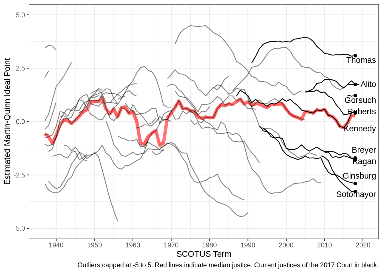
15.6 Chapter 9: Objects and Loops
cen10 <- read_csv("data/input/usc2010_001percent.csv")
sample_acs <- read_csv("data/input/acs2015_1percent.csv")
Checkpoint #3
cen10 %>%
  group_by(state) %>%
  summarise(avg_age = mean(age)) %>%
  arrange(desc(avg_age)) %>%
  slice(1:10)
## `summarise()` ungrouping output (override with `.groups` argument)## # A tibble: 10 x 2
## state avg_age
## <chr> <dbl>
## 1 West Virginia 44.1
## 2 Maine 42.1
## 3 Florida 41.3
## 4 New Hampshire 41.2
## 5 North Dakota 41.1
## 6 Montana 40.6
## 7 Vermont 40.3
## 8 Connecticut 40.1
## 9 Wisconsin 39.9
## 10 New Mexico 39.3Exercise 2
states_of_interest <- c("California", "Massachusetts", "New Hampshire", "Washington")

for (state_i in states_of_interest) {
  state_subset <- cen10 %>% filter(state == state_i)

  print(state_i)

  print(table(state_subset$race, state_subset$sex))
}
## [1] "California"
##
## Female Male
## American Indian or Alaska Native 21 21
## Black/Negro 127 126
## Chinese 76 65
## Japanese 15 12
## Other Asian or Pacific Islander 182 177
## Other race, nec 283 302
## Three or more major races 7 7
## Two major races 91 83
## White 1085 1083
## [1] "Massachusetts"
##
## Female Male
## American Indian or Alaska Native 4 1
## Black/Negro 21 17
## Chinese 8 7
## Japanese 1 1
## Other Asian or Pacific Islander 14 14
## Other race, nec 9 17
## Two major races 10 8
## White 272 243
## [1] "New Hampshire"
##
## Female Male
## American Indian or Alaska Native 1 0
## Black/Negro 0 1
## Chinese 0 1
## Japanese 1 0
## Other Asian or Pacific Islander 2 1
## Other race, nec 1 0
## Two major races 0 1
## White 66 63
## [1] "Washington"
##
## Female Male
## American Indian or Alaska Native 9 5
## Black/Negro 11 9
## Chinese 2 7
## Japanese 4 0
## Other Asian or Pacific Islander 28 18
## Other race, nec 19 18
## Three or more major races 0 2
## Two major races 17 16
## White 267 257Exercise 3
race_d <- c()
state_d <- c()
proportion_d <- c()
answer <- data.frame(race_d, state_d, proportion_d)
Then
for (state in states_of_interest) {
  for (race in unique(cen10$race)) {
    race_state_num <- nrow(cen10[cen10$race == race & cen10$state == state, ])
    state_pop <- nrow(cen10[cen10$state == state, ])
    race_perc <- round(100 * (race_state_num / (state_pop)), digits = 2)
    line <- data.frame(race_d = race, state_d = state, proportion_d = race_perc)
    answer <- rbind(answer, line)
  }
}
15.7 Chapter 11: Demoratic Peace Project
Task 1: Data Input and Standardization
mid_b <- read_csv("data/input/MIDB_4.2.csv")
polity <- read_excel("data/input/p4v2017.xls")
Task 2: Data Merging
mid_y_by_y <- data_frame(ccode = numeric(),
                               year = numeric(),
                               dispute = numeric())
colnames(mid_b)
for(i in 1:nrow(mid_b)) {
    x <- data_frame(ccode = mid_b$ccode[i], ## row i's country
    year = mid_b$styear[i]:mid_b$endyear[i],  ## sequence of years for dispute in row i
    dispute = 1)## there was a dispute
    mid_y_by_y <- rbind(mid_y_by_y, x)
}

merged_mid_polity <- left_join(polity,
                 distinct(mid_y_by_y),
                 by = c("ccode", "year"))
Task 3: Tabulations and Visualization
#don't include the -88, -77, -66 values in calculating the mean of polity
mean_polity_by_year <- merged_mid_polity %>% group_by(year) %>% summarise(mean_polity = mean(polity[which(polity <11 & polity > -11)]))

mean_polity_by_year_ordered <- arrange(mean_polity_by_year, year)

mean_polity_by_year_mid <- merged_mid_polity %>% group_by(year, dispute) %>% summarise(mean_polity_mid = mean(polity[which(polity <11 & polity > -11)]))

mean_polity_by_year_mid_ordered <- arrange(mean_polity_by_year_mid, year)

mean_polity_no_mid <- mean_polity_by_year_mid_ordered %>% filter(dispute == 0)
mean_polity_yes_mid <- mean_polity_by_year_mid_ordered %>% filter(dispute == 1)


answer <- ggplot(data = mean_polity_by_year_ordered, aes(x = year, y = mean_polity)) +
  geom_line() +
  labs(y = "Mean Polity Score",
       x = "") +
  geom_vline(xintercept = c(1914, 1929, 1939, 1989, 2008), linetype = "dashed")

answer + geom_line(data =mean_polity_no_mid, aes(x = year, y = mean_polity_mid), col = "indianred") + geom_line(data =mean_polity_yes_mid, aes(x = year, y = mean_polity_mid), col = "dodgerblue")
15.8 Chapter 12: Simulation
15.8.1 Census Sampling
pop <- read_csv("data/input/usc2010_001percent.csv")## Parsed with column specification:
## cols(
## state = col_character(),
## sex = col_character(),
## age = col_double(),
## race = col_character()
## )mean(pop$race != "White")## [1] 0.2806517set.seed(1669482)
samp <- sample_n(pop, 100)
mean(samp$race != "White")## [1] 0.22ests <- c()
set.seed(1669482)
for (i in 1:20) {
samp <- sample_n(pop, 100)
ests[i] <- mean(samp$race != "White")
}
mean(ests)pop_with_prop <- mutate(pop, propensity = ifelse(race != "White", 0.9, 1))ests <- c()
set.seed(1669482)
for (i in 1:20) {
samp <- sample_n(pop_with_prop, 100, weight = propensity)
ests[i] <- mean(samp$race != "White")
}
mean(ests)ests <- c()
set.seed(1669482)
for (i in 1:20) {
samp <- sample_n(pop_with_prop, 10000, weight = propensity)
ests[i] <- mean(samp$race != "White")
}
mean(ests)