2 Interactive Jobs

When you first log on to the RCE you are on a login node. The login nodes are not designed for intensive computation; the purpose of the login nodes is to provide access to the interactive nodes and the batch nodes. Interactive jobs are useful when a) you need a lot of memory (e.g., because you need to load a large dataset into memory), and/or b) you want to use multiple cores to speed up your computation.

2.1 Launching applications

Running applications on the interactive nodes is very easy; just log in using NoMachine and launch your application from the Application --> RCE Powered menu. A dialog will open asking you how much memory you need and how many CPUs, and then your application will open. That’s all there is to it! Well, we should say that the RCE is a shared resource, so please try not to request more memory or CPUs than you need. Also, applications running on the interactive nodes will expire after five days; you can request an extension, but if you fail to do so your job will be terminated 120 hours after it starts.

2.2 Available applications

Available RCE powered applications include:

Gauss
Mathematica
Matlab/Octave
R/RStudio
SAS
Stata (MP and SE)
StatTransfer

Other applications (e.g., Python/IPython, perl, tesseract, various Unix programs and utilities) can be run on the interactive nodes by launching a terminal on an interactive node (Applications --> RCE Powered --> RCE Shell) and launching your program from the command line.

If you are using the interactive nodes primarily for the large memory they provide you should have all the information you need to begin taking advantage of the RCE. If you are also interested in using multiple CPU cores to speed up your computations, read on! The following sections contain examples illustrating techniques for utilizing multiple cores on the RCE.

2.3 Using multiple CPUs

This section illustrates how to take advantage of multiple cores when running interactive jobs on the RCE, with the goal of getting CPU intensive tasks to run faster.

2.3.1 R

Using multiple cores to speed up simulations

Running computations in parallel on multiple cores is often an effective way to speed up computations. This can be especially useful when doing simulations, or when using resampling methods such as bootstrap or permutation tests. In this example parallel processing is used to simulate the sampling distribution of the mean for samples of various sizes.

We start by setting up a helper function to repeatedly generate a sample of a given size and calculate the sample mean.
```
## function to generate distribution of means for a range of sample sizes
meanDist <- function(n, nsamp = 5000) {
  replicate(nsamp, mean(rnorm(n)))
}

## range of sample sizes to iterate over
sampSizes <- seq(10, 500, by = 5)
```
Next iterate over a range of sample sizes, generating a distribution of means for each one. This can be slow because R normally uses only one core:
```
system.time(means <- lapply(sampSizes, meanDist))
```
The simulation can be carried out much more rapidly using mclapply instead:
```
library(parallel)
system.time(means <- mclapply(sampSizes, meanDist, mc.cores = 7))
```
Like lapply the mclapply function returns a list, which we can process as usual. For example, we can construct histograms of the sampling distributions of the mean that we simulated above:
```
## plot the distribution of means at various sample sizes
par(mfrow=c(6, 5), mar = c(0,0,2,2), cex = .7)
for(i in 1:30) {
  hist(means[[i]],
       main = paste("n =",
                    sampSizes[i]),
       axes = FALSE,
       xlim = range(unlist(means)))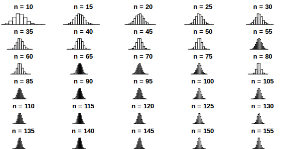
}
```
Using multiple cores to speed up computations

In the previous example we generated the data on each iteration. This kind of simulation can be useful, but often you want to parallelize a function that processes data from a (potentially large) number of files. This is also easy to do using the parallel package in R. In the following example we count number of characters in all the text files in the texlive directory.
```
## List the files to iterate over
textFiles<- list.files("/usr/share/texlive/",
                       recursive = TRUE,
                       pattern = "\\.txt$|\\.tex$",
                       full.names = TRUE)

## function for counting characters (NOTE: this example isn't realistic -- it
## would be better to use the unix "wc" utility if you were doing this
## in real life...)
countChars <-  function(x) {
  sum(nchar(readLines(x, warn = FALSE), type = "width"))
}
```
We have length(textFiles) text files to process. We can do this using a single core:
```
system.time(nchars <- unlist(lapply(textFiles, countChars)))
```
but this is too slow. We can do the computation more quickly using multiple cores:
```
system.time(nchars <- unlist(mclapply(textFiles, countChars, mc.cores = 7)))
```
and calculate the total number of characters in the text files by summing over the result
```
sum(nchars, na.rm = TRUE)
```
For more details and examples using the parallel package, refer to the parallel package documentation or run help(package = "parallel") at the R prompt. For other ways of running computations in parallel refer to the HPC task view.

2.3.2 Python

Running computations in parallel on multiple cores is often an effective way to speed up computations. This can be useful when we want to iterate over a set of inputs, e.g., applying a function to each of a set of files. In this example we count the number of characters in all the files under the texlive directory.

import os
import fnmatch
textFiles = []
for root, dirnames, filenames in os.walk('/usr/share/texlive'):
    for filename in fnmatch.filter(filenames, '*.tex') + fnmatch.filter(filenames, "*.txt"):
        textFiles.append(os.path.join(root, filename))

We have len(textFiles) 2080 text files to process. We can do this using a single core:

import time
start = time.time()

num_chars = 0
for fname in textFiles:
    try:
        with open(fname, 'r') as f:
            for line in f:
                num_chars += len(line)
    except:
        pass

stop = time.time()

It takes around print(stop - start) 1.27 seconds to count the characters in these files, which is aleady pretty fast. But, for even more speed we can use the multiprocessing library to perform the operation using multiple cores:

import multiprocessing

def f(fname):
    num_chars = []
    try:
        with open(fname, 'r') as this_file:
            for line in this_file:
                num_chars.append(len(line))
    except:
        pass
    return sum(num_chars)

start = time.time()

pool = multiprocessing.Pool(7)
nchar = pool.map(f, textFiles)
pool.close()
pool.join()

end = time.time()

which reduces the time to print(end - start) 0.33 seconds.

2.3.3 Other languages

Using multiple CPU cores in Stata, Matlab and SAS does not require explicit activation – many functions will automatically use multiple cores if available. For Matlab user-written code can also take advantage of multiple CPUs using the parfor command. Python uses can run multiple processes using the multiprocessing library.