Plotting and inference for clarify_est objects — plot.clarify

summary() tabulates the estimates and confidence intervals and (optionally) p-values from a clarify_est object. confint() computes confidence intervals. plot() plots the "posterior" distribution of estimates.

Usage

# S3 method for clarify_est
plot(
  x,
  parm,
  ci = TRUE,
  level = 0.95,
  method = "quantile",
  reference = FALSE,
  ncol = 3,
  ...
)

# S3 method for clarify_est
summary(object, parm, level = 0.95, method = "quantile", null = NA, ...)

# S3 method for clarify_est
confint(object, parm, level = 0.95, method = "quantile", ...)

Arguments

parm: a vector of the names or indices of the estimates to plot. If unspecified, all estimates will be displayed.
ci: logical; whether to display confidence interval limits for the estimates. Default is TRUE.
level: the confidence level desired. Default is .95 for 95% confidence intervals.
method: the method used to compute p-values and confidence intervals. Can be "wald" to use a Normal approximation or "quantile" to use the simulated sampling distribution (default). See Details. Abbreviations allowed.
reference: logical; whether to overlay a normal density reference distribution over the plots. Default is FALSE.
ncol: the number of columns used when wrapping multiple plots; default is 3.
...: for plot(), further arguments passed to ggplot2::geom_density().
object, x: a clarify_est object; the output of a call to sim_apply() or its wrappers.
null: the values of the parameters under the null hypothesis for the p-value calculations. Should have length equal to the number of quantities estimated, or one, in which case it will be recycled, or it can be a named vector with just the names of quantities for which null values are to be set. Set values to NA to omit p-values for those quantities. When all values are NA, the default, no p-values are produced.

Value

For summary(), a summary.clarify_est object, which is a matrix containing the coefficient estimates, standard errors, test statistics, p-values, and confidence intervals. Not all columns will be present depending on the arguments supplied to summary().

For confint(), a matrix containing the confidence intervals for the requested quantities.

For plot(), a ggplot object.

Details

summary() uses the estimates computed from the original model as its estimates and uses the simulated parameters for inference only, in line with the recommendations of Rainey (2023).

When method = "wald", the standard deviation of the simulation estimates is used as the standard error, which is used in the z-statistics and the confidence intervals. The p-values and confidence intervals are valid only when the sampling distribution of the resulting statistic is normal (which can be assessed using plot()). When method = "quantile", the confidence interval is calculated using the quantiles of the simulation estimates corresponding to level, and the p-value is calculated as twice the proportion of simulation estimates less than or greater than null, whichever is smaller; this is equivalent to inverting the confidence interval but is only truly valid when the true sampling distribution is only a location shift from the sampling distribution under the null hypothesis and should therefore be interpreted with caution. Using "method = "quantile" (the default) is recommended because the confidence intervals will be valid even if the sampling distribution is not Normally distributed. The precision of the p-values and confidence intervals depends on the number of simulations requested (the value of n supplied to sim()).

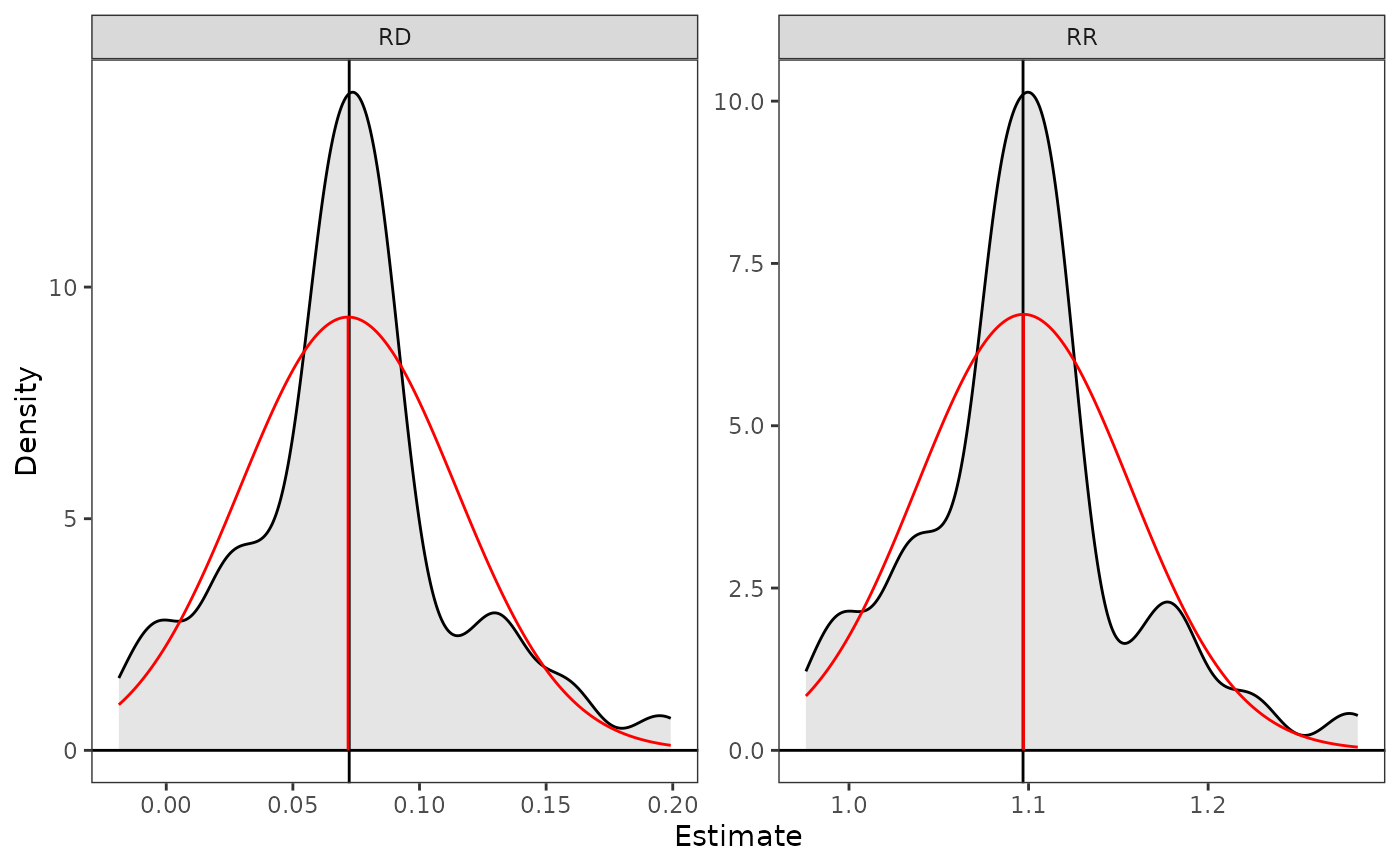
The plots are produced using ggplot2::geom_density() and can be customized with ggplot2 functions. When reference = TRUE, a reference Normal distribution is produced using the empirical mean and standard deviation of the simulated values. A blue references line is plotted at the median of the simulated values. For Wald-based inference to be valid, the reference distribution should overlap with the empirical distribution, in which case the quantile-based and Wald-based intervals should be similar. For quantile-based inference to be valid, the median of the estimates should overlap with the estimated value; this is a necessary but not sufficient condition, though.

References

Rainey, C. (2023). A careful consideration of CLARIFY: Simulation-induced bias in point estimates of quantities of interest. Political Science Research and Methods, 1–10. doi:10.1017/psrm.2023.8

Examples

data("lalonde", package = "MatchIt")
fit <- glm(I(re78 > 0) ~ treat + age + race + nodegree + re74,
          data = lalonde)

s <- sim(fit, n = 100)

# Compute average marginal means for `treat`
est <- sim_ame(s, var = "treat", verbose = FALSE)
coef(est)
#>   E[Y(0)]   E[Y(1)] 
#> 0.7453346 0.8175754 

# Compute average marginal effects on risk difference
# (RD) and risk ratio (RR) scale
est <- transform(est,
                 RD = `E[Y(1)]` - `E[Y(0)]`,
                 RR = `E[Y(1)]` / `E[Y(0)]`)

# Compute confidence intervals and p-values,
# using given null values for computing p-values
summary(est, null = c(`RD` = 0, `RR` = 1))
#>         Estimate   2.5 %  97.5 % P-value
#> E[Y(0)]   0.7453  0.7027  0.7956       .
#> E[Y(1)]   0.8176  0.7584  0.8936       .
#> RD        0.0722 -0.0102  0.1675    0.14
#> RR        1.0969  0.9870  1.2392    0.14

# Same tests using normal approximation and alternate
# syntax for `null`
summary(est, null = c(NA, NA, 0, 1),
        normal = TRUE)
#>         Estimate   2.5 %  97.5 % P-value
#> E[Y(0)]   0.7453  0.7027  0.7956       .
#> E[Y(1)]   0.8176  0.7584  0.8936       .
#> RD        0.0722 -0.0102  0.1675    0.14
#> RR        1.0969  0.9870  1.2392    0.14

# Plot the RD and RR with a reference distribution
plot(est, parm = c("RD", "RR"), reference = TRUE,
     ci = FALSE)


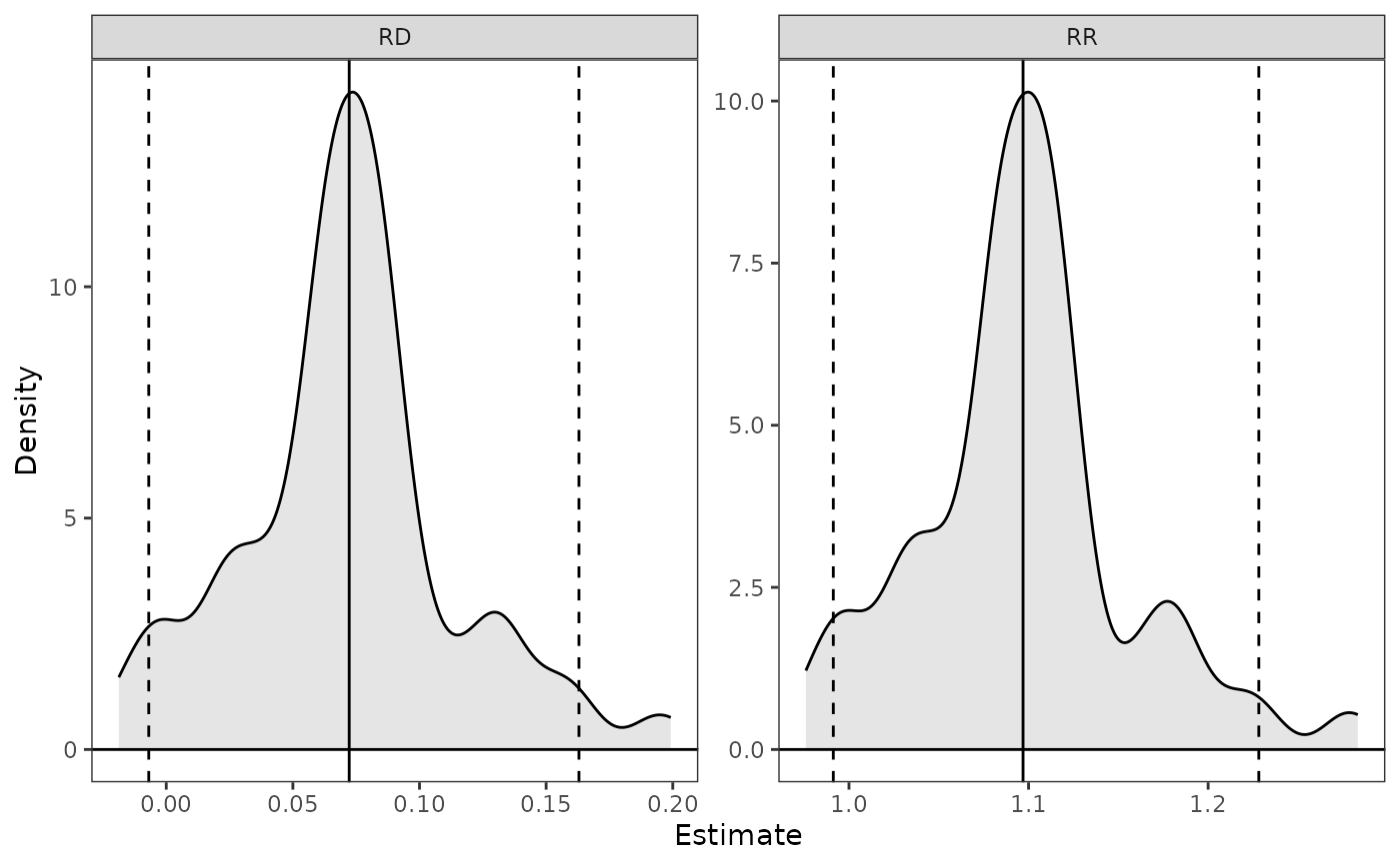
# Plot the RD and RR with quantile confidence bounds
plot(est, parm = c("RD", "RR"), ci = TRUE)

References

Montiel Olea, J. L., & Plagborg-Møller, M. (2019). Simultaneous confidence bands: Theory, implementation, and an application to SVARs. Journal of Applied Econometrics, 34(1), 1–17. doi:10.1002/jae.2656